A previous article shows how to convert a positive integer from base 10 to any other arbitrary base. For example, 15 (base 10) = 120 (base 3) because 15 = 1*32 + 2*31 + 0*30. Representing integers is probably familiar to many readers. But did you know that you can do the same with fractions? This article shows how to convert a decimal value such as (0.021) in base 3 into a fraction. In addition, by using this technique, you can construct a Halton sequence, which can be used to create quasirandom numbers. In a subsequent article, I will show how to construct quasirandom numbers and use them in quasi-Monte Carlo techniques to estimate an integral.
The word "decimal" implies base 10, so radix point is the general name given to the period or dot that separates the integer part of a number from the fractional part of a number. Similarly, a "decimal value" is more properly called a radix fraction. I'll use these fancy terms, but feel free to replace "radix point" with "decimal point" and "radix fraction" with "decimal value" if you prefer.
Represent decimals as fractions in any base
In base 10, a decimal is really a fraction in disguise. A decimal such as 0.123 is a representation of a fraction that uses powers of 10 in the denominator. That is, the decimal 0.456 (base 10) equals 4*10-1 + 5*10-2 + 6*10-3. More generally, a base-10 decimal is a sum of terms \(\Sigma c_{i} 10^{-i}\), where \(c_{i}\) are the digits to the right of the decimal point.
In a similar way, radix fractions in other bases are the sum of fractions that have powers of the base in the denominator. For example:
- In base 2, the radix fraction (0.1101)2 represents the fraction 1*2-1 + 1*2-2 + 0*2-3 + 1*2-4, or 1/2 + 1/4 + 0/8 + 1/16.
- In base 3, the radix fraction (0.0121)3 represents the fraction 0*3-1 + 1*3-2 + 2*3-3 + 1*3-4, or 0/3 + 1/9 + 2*27 + 1/81.
The following SAS IML function (called ConvertFracFromBase) converts a row vector of coefficients (the digits after the radix point) into a fraction in a specified base. In the function, the expression base##pow computes the vector of powers b-1, b-2, and so forth. The elementwise multiplication (#) with the digit vector (c) and the subsequent summation ([,+]) calculates the value of the fraction.
After defining the function, the program shows examples of calling the functions for radix values in base 2 and base 3:
proc iml; /* Convert row vectors from any base to a fraction in base 10. The row vector represents coefficients for a radix fraction in base b. For example: Base 2: c = {1 1 0 1} represents 1/2 + 1/4 + 0/8 + 1/16 Base 3: c = {0 1 2 1} represents 0/3 + 1/9 + 2/27 + 1/81. The input, c, can also be a matrix for which each row c[i,] is a vector of coefficients. */ start ConvertFracFromBase(c, base); pow = -( 1:ncol(c) ); /* decreasing powers */ factor = base##pow; /* b^{-1}, b^{-2}, ... */ fract10 = (c # factor)[ ,+]; /* fractions */ return fract10; finish; /* test the function */ s2 = {1 1 0 1, /* 1/2 + 1/4 + 0/8 + 1/16 */ 0 0 1 1}; /* 0/2 + 0/4 + 1/8 + 1/16 */ f2 = ConvertFracFromBase(s2, 2); print s2[L="" c={'1/2' '1/4' '1/8' '1/16'}], f2[F=FRACT32.]; s3 = {1 2 0 1, /* 1/3 + 2/9 + 0/27 + 1/81 */ 0 2 1 0}; /* 0/3 + 2/9 + 1/27 + 0/81 */ f3 = ConvertFracFromBase(s3, 3); print s3[L="" c={'1/3' '1/9' '1/27' '1/81'}], f3[F=FRACT32.]; |
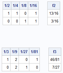
The tables show the coefficients that represent the radix fraction in each base, along with the fractional value. Notice that I used the FRACT. format in SAS to display the floating-point result as a fraction.
The ConvertFracFromBase function is efficient because it uses matrix operations. Instead of looping over digits, it computes the entire set of denominators in a single vector (factor), multiplies them by the corresponding digits, and then sums the resulting products. This vectorization is key to generating the Halton sequence efficiently.
The Halton sequence
If you can convert an integer to any base (from the previous article) and evaluate a radix fraction (from the previous section), then you can construct a Halton sequence. You first specify the base, b, which is typically a prime number. Then, as discussed in the Wikipedia article about the Halton sequence, you construct the Halton sequence of length n as follows.
- Base conversion: Represent the integers 1-n as numbers in base b.
- Digit reflection: Place a radix point at the end of each number and flip or reflect the digits across the radix point to create a set of radix fraction values.
- Convert to base 10: Evaluate these radix fraction values.
For example, in base 2, here is how to construct the first n=7 terms of the Halton sequence:
- The integers in base 2 are represented as 1, 10, 11, 100, 101, 110, 111, 1000, ...
- Reverse the digits by reflecting them across the radix point: 0.1, 0.01, 0.11, 0.001, 0.101, 0.011, 0.111, 0.0001, ...
- Express these radix fraction values as fractions: 1/2, 1/4, 3/4, 1/8, 5/8, 3/8, 7/8, ... You can evaluate these fraction to obtain the base-10 values.
The following SAS IML function carries out this algorithm. The utility function, reverseCols, performs the reversal of the digits from integers to radix fractions. You must first load the ConvertToBase function from a previous article. For convenience, that and all the functions in this article are provided in the Appendix.
/* load ConvertToBase and other functions from first blog post */ load module = _ALL_; /* reverse the order of the columns of a matrix */ start reverseCols(M); return M[, ncol(M):1]; finish; /* generate a Halton sequence for one specified base INPUT: _n : a column vector of integers base : a positive scalar integer, often chosen to be a prime number OUTPUT: a vector of length nrow(_n) that contains a Halton sequence */ start HaltonSeq1( _n, base ); n = colvec(_n); C1 = ConvertToBase(n, base); /* convert integers to base-b digits */ C = reverseCols(C1); /* reverse digits to get fraction coefficients */ return ConvertFracFromBase(C, base); /* convert base-b fraction to base-10 decimal value */ finish; /* test the functions */ n = T(1:10); s2 = HaltonSeq1( n, 2); s3 = HaltonSeq1( n, 3); print n s2[F=FRACT32.] s3[F=FRACT32.]; |
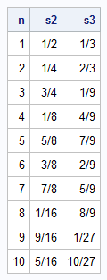
The table shows an interesting property of the fractions in the Halton sequence. At each "level," the fractions uniformly fill the interval [0, 1]. For example:
- In base 2, the first fraction is 1/2, which evenly divide the interval into two subintervals. Then come 1/4 and 3/4, which evenly divide the subintervals from the previous fraction. Then come 1/8, 5/8, 3/8 and 7/8, which evenly subdivide the intervals again.
- In base 3, the first two fractions are 1/3 and 2/3, which evenly divides the interval into three subintervals. Then come the fractions with 9 in the denominator, which evenly divide the subintervals from the previous fraction.
The Halton fractions are deterministic (not random), but their distribution on the unit interval is highly regular. As you increase the number of terms, the points fill the interval more uniformly than truly random numbers do. If n is a power of the base, there are no clusters or gaps with the Halton fractions.
Quasirandom points from the Halton sequence
You can use the Halton sequence to obtain n quasirandom points in the unit cube in d-dimensional space. For each dimension, you choose a (different) prime number as the base. You then generate n points for each dimension and create the Cartesian product of the sequences. For example, to generate points in the unit square in 2-D, you can use b=2 as the base for the first dimension and b=3 as the base for the second dimension.
The following statements generate n=100 points in base 2 and 3, then display a scatter plot of the resulting Cartesian product in 2-D:
/* 2-D quasirandom points */ n = T(1:100); s2 = HaltonSeq1( n, 2); s3 = HaltonSeq1( n, 3); title "Halton QuasiRandom Values"; call scatter(s2,s3) grid={x y} label={'x' 'y'} procopt="aspect=1"; |
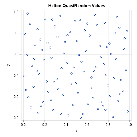
The scatter plot shows an important property of the ordered pairs in the unit square. As discussed previously, the Halton points are evenly spaced. As you add more and more points, the new points fill one of the larger gaps between points. This property makes them a popular choice for numerical quasi-Monte Carlo integration, which I will discuss in a future article.
Summary
This article discussed some functions that enable you to generate Halton sequences. These sequences are useful for quasi-Monte Carlo integration. The Appendix contains the complete set of SAS IML functions that are used for this purpose. A future article shows how to use these functions to estimate a definite integral by using quasi-Monte Carlo integration.
Appendix: SAS IML functions for base conversion and Halton sequences
The following IML statements define and store the functions used in this and a previous article. You can use the LOAD statement to use these functions in your own programs.
/* APPENDIX: A set of SAS IML functions that generate quasirandom points in d dimensions by using Halton sequences */ proc iml; /* Compute LOG_b(x) for a vector of x values and for an integer base, b > 0. If an input value is not positive, this function returns a missing value. Computers represent numbers internally in base b=2, so use the change-of-base formula log_b(x) = log2(x) / log2(b) to compute the logarithm in any base, b. */ start logbase(x, base=10); if all(x)>0 then return log2(x) / log2(base); /* otherwise, return missing values for x <= 0 */ y = j(nrow(x), ncol(x), .); idx = loc(x>0); if ncol(idx)>0 then y[idx] = log2(x[idx]) / log2(base); return y; finish; /* This function returns the number of digits in the base-b representation of an integer, x. If n >= 0 is a base-10 integer, it has k = ceil(log_b(n+1)) digits when represented in base b. See https://blogs.sas.com/content/iml/2015/08/31/digits-in-integer.html */ start numDigBase(x, base=10); n = round(x); /* ensure argument is an integer */ return ceil( logbase(n+1,base) ); finish; /* Convert integer x > 0 to a row vector in base b. If x is a column vector, return a matrix where each row is the base-b representation of x[i]. The most significant bit is to the left; the least significant bit is to the right. For example, n=15 and base=3 gives (120)_3 because 15 = 1*3##2 + 2*3##1 + 0*3##0. */ start ConvertToBase(x, base); n = round(x); /* ensure inputs are integers */ numDig = numDigBase(max(n), base); /* For an explanation, see https://blogs.sas.com/content/iml/2015/08/31/digits-in-integer.html */ c = j(nrow(n), numDig, 0); do i = 1 to numDig; a = mod(n, base); n = floor( n/base ); c[ , numDig - i + 1] = a; end; return c; finish; /* Convert row vectors from any base to a fraction in base 10. The row vector represents coefficients for a fraction in base b. For example: Base 2: c = {1 1 0 1} represents 1/2 + 1/4 + 0/8 + 1/16 Base 3: c = {0 1 2 1} represents 0/3 + 1/9 + 2/27 + 1/81. The input, c, can also be a matrix for which each row c[i,] is a vector of coefficients. */ start ConvertFracFromBase(c, base); pow = -( 1:ncol(c) ); /* decreasing powers */ factor = base##pow; /* b^{-1}, b^{-2}, ... */ fract10 = (c # factor)[ ,+]; /* fractions */ return fract10; finish; /* reverse the order of the columns of a matrix */ start reverseCols(M); return M[, ncol(M):1]; finish; /* generate a Halton sequence for a specified base INPUT: _n : a column vector of integers base : a positive scalar integer, often chosen to be a prime number OUTPUT: a vector of length nrow(_n) that contains a Halton sequence */ start HaltonSeq1( _n, base ); n = colvec(_n); C1 = ConvertToBase(n, base); C = reverseCols(C1); return ConvertFracFromBase(C, base); finish; store module=( logbase numDigBase ConvertToBase ConvertFromBase reverseCols ConvertFracFromBase HaltonSeq1 ); QUIT; |
