When I encounter a new function, I usually graph it to gain intuition about how the function transforms its inputs. Recently, I needed to use the Rayleigh quotient function, which is connected to the estimation of eigenvalues and eigenvectors for symmetric matrices. It has been several years since I last thought about the Rayleigh quotient, so this article shows how to visualize the function in SAS for 2 x 2 and 3 x 3 symmetric matrices.

What is the Rayleigh quotient?

The Rayleigh quotient is a tool in linear algebra that is useful for understanding the eigenvalues and eigenvectors of a symmetric matrix. For an n x n symmetric matrix, A, the Rayleigh quotient is the scalar function
     $R_A(x) = \frac{x^\prime A x}{x^\prime x} = \frac{x^\prime A x}{\Vert x \Vert^2}$
for any n x 1 nonzero vector, x.

The Rayleigh quotient measures how much the matrix A stretches nonzero vectors. Notice that the Rayleigh quotient simplifies when x has unit length: $R_A(x) = x^\prime A x$ when ||x||=1. In this form, the Rayleigh quotient tells you how much A stretches a unit vector in any direction.

The question of "how much a matrix stretches a vector," naturally leads to eigenvalues and eigenvectors. Recall that the eigenvalues of a symmetric matrix are real. The Rayleigh Theorem states that the range of the Rayleigh quotient function has the following properties:

• If λ₁ ≥ λ₂ ≥ ... ≥ λ_n are the eigenvalues of A in decreasing order, then λ₁ ≥ R_A(x) ≥ λ_n for every nonzero vector, x. (Note: In this article, λ₁ is the largest eigenvalue. Some references reverse the notation and use λ_n as the largest eigenvalue.)
• The maximum value of R_A(x) is largest eigenvalue, λ₁, which is attained when x is the eigenvector corresponding to λ₁.
• The minimum value of R_A(x) is smallest eigenvalue, λ_n, which is attained when x is the eigenvector corresponding to λ_n.

This blog post uses SAS to create graphs that illustrate the Rayleigh Theorem for 2 x 2 and 3 x 3 symmetric matrices.

Visualize the Rayleigh quotient for 2x2 symmetric matrices

Let's choose a specific 2 x 2 symmetric matrix and graph the Rayleigh quotient function for every unit vector. In statistics, we are often interested in eigenvalues of correlation matrices, so let's choose the matrix A to be the correlation matrix with correlation 0.5. You can use the EIGEN subroutine in PROC IML to compute the eigenvalues and eigenvectors, as follows:

proc iml;
A = {1   0.5,
     0.5 1  };
call eigen(D, U, A);
print D[L="Eigenvalues" r=(1:2)], 
      U[c={'Eigenvector 1' 'Eigenvector 2'}];

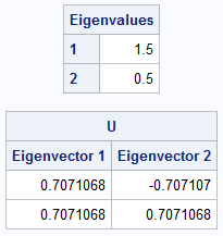
The largest eigenvalue is 1.5 and the smallest is 0.5. The corresponding eigenvectors are (sqrt(2), sqrt(2)) and (-sqrt(2), sqrt(2)), respectively. From trigonometry, you probably already know the angles that these vectors make with the X axis (π/4 and 3π/4), but let's use the ATAN2 function in SAS to compute the angles in the interval (-π, π):

Radians = atan2(U[2,], U[1,]);                  /* in (-pi/2, pi/2]. Note: syntax is ATAN2(y,x) */
pi = constant('pi');
Radians = choose(Radians < 0, Radians + pi, Radians); /* in (0, pi] */
print Radians[c={'theta 1' 'theta 2'}];
Degrees = 180/pi * Radians;
optimum = Radians` || Degrees`;
print optimum[r={'Eigenvector 1' 'Eigenvector 2'} c={'Radians' 'Degrees'} F=BEST6.];

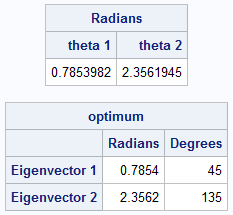
As we already know, the angles of the eigenvectors are equal to π/4 and &3π/4. Of course, if v is an eigenvector, then so is -v, so the SAS code standardizes the angles to lie in the interval (0, π]. The output contains both the radian and the degree measures of the angles.

Let's use the Rayleigh quotient function to obtain these same results. According to the Rayleigh Theorem, if we graph the Rayleigh quotient function on the unit circle, the maximum value of the function should be 1.5 for the input angle π/4. Similarly, the minimum value of the function should be 0.5 for the input angle 3π/4. The following statements evaluate the Rayleigh quotient for unit vectors whose angle with the X axis in [0, 2π]:

/* write a loop (yes, this loop can be vectorized!) */
theta = do(0, 2*pi, pi/41);
x = cos(theta) // sin(theta);  /* each column is a vector on the unit circle */
R = j(1, ncol(theta), .);
do i = 1 to ncol(theta);
   v = x[,i];
   R[i] = v` * (A*v);      /* note |v| = 1 */
end;
 
title "Rayleigh Quotient for 2-D Matrix";
refstmt = "refline " + rowcat(char(Radians,8,4)) + 
          "/axis=x lineattrs=(color=DarkRed) label=('pi/4' '3 pi/4');";
call series(theta, R) grid={x,y} other=refstmt xvalues=0:6;

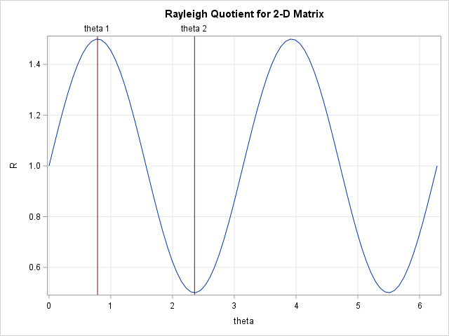
As predicted, the graph of the Rayleigh quotient function attains its maximum and minimum values at π/4 and 3π/4. The height of the function at those points are 1.5 and 0.5, which are the largest and smallest eigenvalues, respectively, for A. Notice that we could have saved some computations by evaluating the Rayleigh function only on a half-circle. The Rayleigh quotient on [π, 2π] is identical to the quotient on [0, π].

Visualize the Rayleigh quotient for 3x3 symmetric matrices

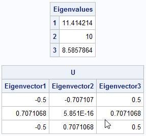
We can perform a similar visualization for a 3 x 3 symmetric matrix. In this case, we want to evaluate the Rayleigh quotient function on the unit sphere. and graph the Rayleigh quotient function for every unit vector. In statistics, we are often interested in eigenvalues of a structured covariance matrix, so let's choose the matrix A to be the following covariance matrix. You can use the EIGEN subroutine in PROC IML to compute the eigenvalues and eigenvectors, as follows:

proc iml;
A = {10 -1  0,
     -1 10 -1,
      0 -1 10};
call eigen(D, U, A);
print D[L="Eigenvalues" r=(1:3)], 
      U[c=('Eigenvector 1':'Eigenvector 3')];

Step 1: Find the angles for the eigenvectors

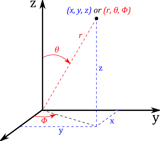
While not strictly necessary, let's find the angles that these vectors make with certain reference vectors. You can do this by using spherical coordinates: to each vector you can associate two angles θ and φ.

There are two competing definitions for these angles: the "physics" convention and the "mathematics" convention. According to the Wikipedia page about spherical coordinates, the physics convention is the ISO standard (Boo! Hiss! Mathematicians were robbed!). In the ISO standard:

• The angle θ is called the inclination angle. It is measured from the z axis. Its value is in the range [0, π].
• The angle φ is called the azimuthal angle. It is measured from the x axis. Its value is in the range [0, 2π].

You can convert a vector from Cartesian to spherical coordinates. The following IML function converts each unit eigenvector (which are the columns in the U matrix) to (θ, φ) values:

/* Find the angles for the eigenvectors in spherical coordinates.  
   Use the symbols and convention for the PHYSICS Convention (ISO standard) from 
   https://en.wikipedia.org/wiki/Spherical_coordinate_system#Cartesian_coordinates
   theta = inclination from z axis in [0, pi]
   phi = azimuthal angle from x axis in [0, 2*pi]
*/
start Vec3DToAngles(M);
   angles = j(ncol(M), 2);
   do i = 1 to ncol(M);
      w = M[,i];
      r = sqrt(w[1]##2+w[2]##2);
      theta = arcos(w[3]);        /* theta = inclination angle */
      phi =  atan2(w[2], w[1]);  /* phi = azimuthal angle */
      angles[i,] = theta || phi;
   end;
   return angles;
finish;
 
evec_angles = Vec3DToAngles(U);
print evec_angles[r=(1:3) c={'theta' 'phi'} F=BEST6.];
pi = constant('pi');
deg = 180/pi * evec_angles;
print deg[r=(1:3) c={'theta (Deg)' 'phi (Deg)'} F=BEST6.];
/* save eigenvector angles to data set */
eigen = D || evec_angles;
create Angles from eigen[c={'Eigenvalue' 'e_theta' 'e_phi'}];
append from eigen;
close;

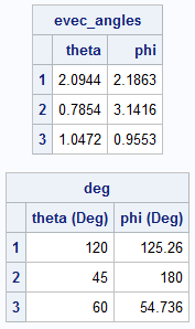
The angles are shown. They are also written to a SAS data set called ANGLES so that they can be used in the visualization of the Rayleigh quotient function. The Rayleigh quotient function will have its maximum value at the angles that correspond to the first eigenvector. It will have its minimum value at the angles that correspond to the third eigenvector.

Step 2: Evaluate the Rayleigh quotient on the unit sphere

Now for the main part of the visualization: evaluate the Rayleigh quotient for a set of vectors on the unit sphere in 3-D. The easiest way to do this is to create a uniform grid of (θ, φ) values and use them to create unit vectors. The vectors are not uniformly spaced in the sphere, but that's okay.

/* generate points on unit sphere in 3-D */
nTheta = 41;
nPhi = 41;
pi = constant('pi');
/* Convert angles to unit vectors by using the PHYSICS Convention (ISO standard) from 
   https://en.wikipedia.org/wiki/Spherical_coordinate_system#Cartesian_coordinates
   theta = inclination from z axis in [0, pi]
   phi = azimuthal angle from x axis in [0, 2*pi]
*/
thetaSeq = do(0, pi, pi/(nTheta-1));    /* theta in [0, pi] */
phiSeq   = do(0, 2*pi, 2*pi/(nPhi-1));  /* phi in [0, 2*pi] */
angle = expandgrid(phiSeq, thetaSeq);
 
/* write a loop to evaluate unit vectors with given angles */
phi   = rowvec(angle[,1]);
theta = rowvec(angle[,2]);
/* each column of X is a unit vector in 3-D */
X = sin(theta) # cos(phi) // /* x-coordinate */
    sin(theta) # sin(phi) // /* y-coordinate */
    cos(theta);              /* z-coordinate */
/* evaluate the Rayleigh quotient on each unit vector */
R = j(nrow(angle), 1, .);
do i = 1 to nrow(angle);
   v = X[,i];
   R[i] = v` * (A*v);
end;
 
results = angle || R;
create Rayleigh from results[c={'phi' 'theta' 'R'}];
append from results;;
close;
QUIT;

The program writes the spherical angles and the Rayleigh quotients to a SAS data set.

Step 3: Visualize the Rayleigh quotient

We can use a heat map to visualize the Rayleigh quotient on the unit sphere by using φ and θ as coordinate axes and by using color to represent the Rayleigh quotient. For the 2-D visualization, I let the ODS graphics system create the tick positions on the axes. For this visualization, I created custom tick positions so that the tick marks have radian values that are fractions of π. If you prefer, you could add tick marks that show the angles in degrees.

data All;
   set Rayleigh Angles;
   label R = "Rayleigh Quotient";
   format Eigenvalue Best4.;
run;
 
/* add custom tick marks. See
   https://blogs.sas.com/content/iml/2020/03/23/custom-tick-marks-sas-graph.html  */
title "Rayleigh Quotient for Vectors on the Unit Sphere";
proc sgplot data= All noautolegend aspect=1;
   heatmapparm x=phi y=theta colorresponse=R / transparency=0.2 name="hm";
   scatter x=e_phi y=e_theta / markerattrs=(symbol=CircleFilled size=12) datalabel=Eigenvalue;
   xaxis grid values=(0.00 0.79 1.57 2.36 3.14 3.93 4.71 5.50 6.28)
       valuesdisplay=('0' 'pi/4' 'pi/2' '3pi/4' 'pi' '5pi/4' '3pi/2' '7pi/4' '2pi');
   yaxis grid values=(0.00 0.79 1.57 2.36 3.14) 
       valuesdisplay=('0' 'pi/4' 'pi/2' '3pi/4' 'pi');
   gradlegend / title="Rayleigh Quotient";
run;

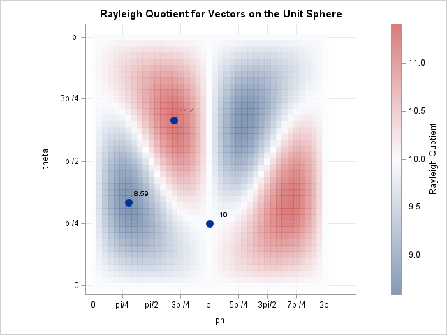
The graph confirms the properties of the Rayleigh quotient:

• The Rayleigh quotient is always in the range [8.56, 11.4] because 8.56 is the smallest eigenvalue of A and 11.4 is the largest eigenvalue.
• The maximum value occurs for the angle that corresponds to the largest eigenvector. Because eigenvectors are not unique, there is also a maximum for the "negative direction". Recall that in spherical coordinates, (-r, φ, θ) = (r, π+φ, π/2-θ). That is why there is a second dark-red region on the heat map.
• The minimum value occurs for the angle that corresponds to the smallest eigenvector. There is also a minimum (dark-blue region) for the "negative direction".
• The middle eigenvector is not an extremum for the Rayleigh quotient. It is on the level set for R_A(x) = 10.

Summary

The Rayleigh quotient is a tool in linear algebra that is associated with eigenvalues and eigenvectors of symmetric matrices. For 2 x 2 symmetric matrices, you can visualize the Rayleigh quotient by evaluating it on the unit circle. For 3 x 3 symmetric matrices, you can evaluate it on the unit sphere. Both methods enable you to visualize the important theoretical properties of the Rayleigh quotient:

• The maximum value is the largest eigenvalue. It achieves its maximum value for the corresponding largest eigenvector.
• The minimum value is the smallest eigenvalue. It achieves its minimum value for the corresponding smallest eigenvector.

Appendix: is it the Raleigh quotient or the Rayleigh quotient?

I live near the city of Raleigh, North Carolina, so I feel compelled to point out that there are two different English noblemen with similar names: