The power method is a well-known iterative scheme to approximate the largest eigenvalue (in absolute value) of a symmetric matrix. It is useful in practice when you need only the largest eigenvalue and eigenvector of a large matrix. The method requires only matrix-vector multiplication and vector scaling.

There is a similar algorithm that can find the smallest eigenvalue and eigenvector of a matrix. The generic name for the algorithm is the inverse power method, although this article describes a variant that is known as Rayleigh quotient iteration because it uses the Rayleigh quotient, which tells you how much a matrix stretches unit vectors in an arbitrary direction. This article implements the inverse power method in SAS IML.

For simplicity, the algorithm in this article assumes that the matrix is not only symmetric but also positive definite. The most important matrices in statistics are correlation and covariance matrices, which are symmetric and positive definite (SPD). An SPD matrix has strictly positive eigenvalues. Thus, in this article, we assume that the eigenvalues are real and that there is a dominant eigenvalue: λ₁ > λ₂ ≥ ... ≥ λ_n > 0.

A 3x3 example matrix

To illustrate the power method and the inverse power method, let's define a small matrix and use the CALL EIGEN subroutine in PROC IML to compute the largest and smallest eigenvalues and the associated eigenvectors:

proc iml;
A = {10 -1  0,
     -1 10 -1,
      0 -1 10};
call eigen(D, U, A);
print D[r=(1:3) F=BEST6.], U[c=('e1':'e3') F=BEST6.];

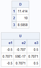
The largest eigenvalue is λ₁ = 11.4; the associated eigenvector is the first column of the U matrix. The smallest eigenvalue is λ₃ = 8.59; the associated eigenvector is the last column of the U matrix.

A review of the power method

Let's quickly review the power method to find the largest eigenvalue and eigenvector. For brevity, I will use the phrase, "the largest eigenvector," instead of the longer phrase, "the eigenvector associated with the largest eigenvalue." A previous article discusses the details of the power method, but it is convenient to present the algorithm here so that you can easily compare it to the inverse power method:

/* The power method for finding the largest eigenvalue and eigenvector.
   The arguments are:
    v         Upon input, contains an initial guess for the largest eigenvector. 
              Upon return it contains an approximation to the largest eigenvector.
    A         The symmetric matrix whose largest eigenvalue is desired. 
    maxIters  The maximum number of iterations. Default=100
    tolerance Relative convergence criterion. Default=1E-6
 
   This implementation assumes that the largest eigenvalue is positive.
*/
start PowerMethod(v, A, maxIters=100, tolerance=1e-6);
   v = v / norm( v );         /* normalize */
   lambdaOld = -1E6;
   do iteration = 1 to maxIters;
      z = A*v;                /* transform v_i */
      v = z / norm( z );      /* normalize to get v_{i+1} */
      lambda = v` * z;        /* eigenvalue estimate: could use Rayleigh quotient, but more efficient to use v`*z */
      if abs((lambda - lambdaOld)/lambda) < tolerance then 
         return ( lambda );
      lambdaOld = lambda;
   end;
   msg = "WARNING: Power method did not converge after " + char(maxIters) + " iterations.";
   print msg;
   return ( . ); /* no convergence */
finish;
 
/* test the power method on the matrix A */
vL = j(ncol(A),1,1);           /* initial guess eigenvector */
evalL = PowerMethod(vL, A);    /* overwrites vL with estimate for largest eigenvector */
print evalL[c={'Largest Eval'} F=BEST6.];
print vL[c={'Largest Evec'} F=BEST6.];

The program first defines the PowerMethod function, which implements the power method to find the largest eigenvalue and eigenvector. Inside the iteration loop, the program updates the previous eigenvector estimate (v_i) with a new estimate (v_i+1) by doing the following step:

1. Apply the linear operator, A, to v_i, which is the previous estimate.
2. Normalize the result to get v_i+1.
3. Estimate the amount by which A stretches v_i. This estimate uses a hybrid variation of the Rayleigh quotient.

To test the function, the program creates an initial guess for the largest eigenvector, which I chose to be the vector {1,1,1}. The call to the PowerMethod function returns an estimate for the largest eigenvalue and overwrites the initial guess with the estimate for the associated eigenvector. If you compare the output with the results from the EIGEN subroutine, you can see that the power estimates are close. Recall that eigenvectors are not unique. If v is an eigenvector, then so is -v. For this example, the eigenvector returned by the power iteration is the negative of the vector in the first column of U.

The inverse power method

We've assumed that the matrix A has eigenvalues λ₁ > λ₂ ≥ ... ≥ λ_n > 0. Because A does not have a zero eigenvalue, it is nonsingular. Therefore, the matrix A^-1 exists. The eigenvalues for A^-1 are known (from theory) to be {1/λ₁, 1/λ₂, ...,1/λ_n}.

For a numerical analyst, it is anathema to compute an inverse matrix explicitly. Fortunately, you don't have to! The power method algorithm needs to compute the product w = A^-1 v for any vector v. You can find w efficiently by solving the linear system A*w = v for w. Consequently, the inverse power method can be written as follows:

/* If the inverse power method converges, the function returns the smallest eigenvalue. 
   The associated eigenvector is returned in the first argument, v.
 
   If the inverse power method does not converge, the function returns a missing value.
 
   The arguments are:
    v         Upon input, contains an initial guess for the smallest eigenvector. 
              Upon return it contains an approximation to the smallest eigenvector.
    A         The matrix whose largest eigenvalue is desired. 
    maxIters  The maximum number of iterations. Default=100
    tolerance Relative convergence criterion.
 
   This implementation assumes that the smallest eigenvalue is positive.
*/
start InvPowerMethod(v, A, maxIters=100, tolerance = 1e-6);
   v = v / norm( v );  /* normalize */
   lambda = -1E6;
   do iteration = 1 to maxIters;
      lambdaOld = lambda;
      /* Solve linear system A*z = v for z,
         This is equivalent to z = inv(A)*v but is more efficient. */
      z = solve(A, v);       /* inverse transformation */
      v = z / norm(z);       /* normalize z to get new v */
      lambda = v` * A * v;   /* eigenvalue estimate is the Rayleigh quotient */
      if abs((lambda - lambdaOld)/lambda) < tolerance then 
         return ( lambda );
   end;
   msg = "WARNING: Inverse power method did not converge after " + char(maxIters) + " iterations.";
   print msg;
   return ( . ); /* no convergence */
finish;
 
/* test the inverse power method on the matrix A */
vS = j(ncol(A),1,1);             /* initial guess eigenvector */
evalS = InvPowerMethod(vS, A);   /* overwrites vS with estimate for smallest eigenvector */
print evalS[c={'Smallest Eval'} F=BEST6.];
print vS[c={'Smallest Evec'} F=BEST6.];

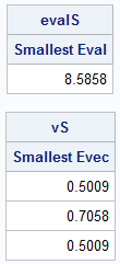
Again, the output agrees with the output from the EIGEN subroutine. (This time, the eigenvectors point in the same direction.) Notice that the IML statements inside the InvPowerMethod function are almost exactly the same as for the (forward) power method except for two lines: the transformation and the estimation of the eigenvalue. You can use the Rayleigh quotient in the (forward) power method, in which case the methods differ only in the choice of a linear transformation: Forward iteration by A or inverse iteration by A^-1.

Convergence of the power methods

Textbooks and Wikipedia prove that the power method converges geometrically with the ratio |λ₂ / λ₁|. Thus, the method converges faster when there is a large gap between the dominant eigenvalue (λ₁) and the next eigenvalue.

The same is true for the inverse power iteration. The convergence of the inverse method depends on the ratio between 1/λ_n-1 and 1/λ_n, which simplifies to the ratio |λ_n/λ_n-1|.

Let's run an example to examine the convergence. Recall that you can construct an arbitrarily large SPD matrix by using a Toeplitz matrix. Let's construct a 50x50 correlation matrix and look at the smallest eigenvalues:

/* Construct SPD matrix:
   https://blogs.sas.com/content/iml/2015/09/23/large-spd-matrix.html
*/
n = 50;                          /* size of matrix */
h = 1/n;                         /* stepsize for decreasing sequence */
v = do(1, h, -h);                /* {1, 5/6, 4/6, ..., 1/6} */
A = toeplitz(v);                 /* PD correlation matrix */
eval = eigval(A);
k = (n-1) || n; 
r = eval[n] / eval[n-1];
print (eval[k])[r=k L="Eigenvalues"];
print r;

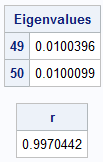
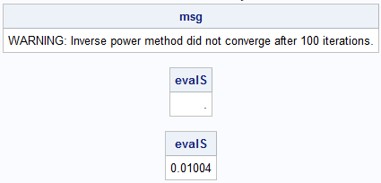
The ratio between the two smallest eigenvalues is 0.997, which is very close to 1. The expression r^k converges to 0 very slowly, which means that it will take many iterations for the inverse power method to converge for this example. The following statements show that the inverse power method does not converge after 100 iterations, which is the default. However, you can increase the number of iterations and call the function repeatedly until you obtain convergence:

v0 = j(ncol(A),1,1);
vS = v0;
evalS = InvPowerMethod(vS, A);        /* default is maxIter=100 */
print evalS;                          /* did not converge! */
 
evalS = InvPowerMethod(vS, A, 1000);  /* reuse vS; increase maxIter parameter */
print evalS;

Summary

This article reviews the power method for finding the largest eigenvalue and eigenvector of a symmetric positive definite matrix, such as a correlation or covariance matrix. The method uses only matrix multiplication. It requires a dominant eigenvalue and converges according to the size of the gap between the largest and second-largest eigenvalues. The algorithm can be modified to compute the smallest eigenvalue and eigenvector. Instead of performing a matrix multiplication at each step, the inverse power method solves a linear system, which is equivalent to multiplying by the matrix inverse. The article shows that the convergence depends on the ratio between the two smallest eigenvalues.

The power methods also work when the dominant eigenvalue is negative, but it's a little trickier to determine convergence because the direction of the vector in the iteration alternates along the eigenspace. One solution is to perform TWO linear transformations for each iteration step. Then the algorithm works regardless of the sign of the dominant eigenvalue.