A previous article describes how to use SAS to find the inflection points of a 1-D function that you can evaluate at any point. The function must be given by a formula (or by an algorithm) because the root-finding algorithm needs to evaluate the function at arbitrary locations. However, sometimes a function is known only at a finite set of points. This situation arises frequently in statistics. For example, a nonparametric regression curve does not have a simple closed-form expression. Neither does a nonparametric density function. Although these functions do not have an explicit formula, you can still use techniques from numerical analysis to approximate points where the first or second derivative of the function vanishes.

For brevity, this article uses the term discrete function instead of the more precise phrase, "a function that is known at only finitely many points." I have previously shown how to approximate extrema for a discrete function. This article shows how to approximate inflection points where the second derivative of the function is zero.

Data and a nonparametric smoother

My previous article found extrema for a loess regression smoother for the Sashelp.ENSO data. I'll once again use the ENSO data, but this time I'll fit a thin-plate spline smoother and evaluate the smoother at a grid of points. The following call to PROC TPSPLINE fits and visualizes the regression model:

/* Create DATA VIEW where x is the independent variable and y is the response */
data Have / view=Have;
set Sashelp.Enso(rename=(Month=x Pressure=y));
keep x y;
run;
/* Evaluate the model and estimate derivatives at these points */
data Grid;
do x = 1 to 36 by 0.5;   
   output;
end;
run;
 
proc tpspline data=Have plots(only)=fitplot;
   model y = (x);
   score data=Grid out=predOut pred;
run;

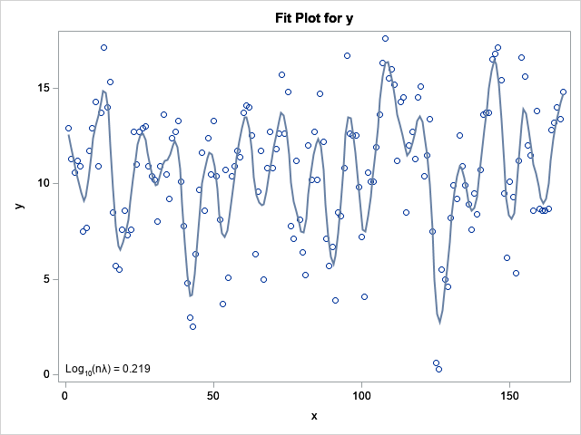
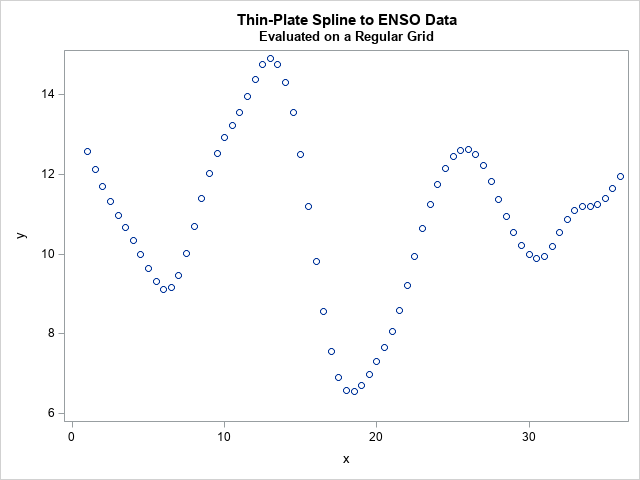
The graph shows the raw data and the thin-plate spline smoother. The smoother has about 25 extrema for x in the interval [1,168], so it will have at least that many inflection points. That is too many for an example, so I scored the regression curve only for x in the range [1, 36], which will enable us to use a curve that has a smaller number of inflection points. The following SAS procedures visualize the regression curve, which is known at 71 discrete locations:

data InData;
set PredOut;
y = p_y;     /* rename the predicted values */
keep x y;
run;
 
title "Thin-Plate Spline to ENSO Data";
title2 "Evaluated on a Regular Grid";
proc sgplot data=InData;
  scatter x=x y=y;
run;

A numerical approximation of a second derivative

The function is known only at a discrete set of (x,y) values. There are several finite-difference formulas that you can use to approximate first and second derivatives. I will use a central difference formula that is used by the NLPFDD function in SAS IML.

proc iml;
/* finite-difference approximation of the second derivative for a 
   function that is known only at discrete points (x[i], y[i]) */
start FDD2(x, y);
   h = dif(x);
   ym2 = lag(y, -2);      /* y[i-2] */
   ym1 = lag(y, -1);      /* y[i-1] */
   yp1 = lag(y,  1);      /* y[i+1] */
   yp2 = lag(y,  2);      /* y[i+2] */
   D2f = (-yp2 + 16*yp1 - 30*y + 16*ym1 - ym2) / (12*h##2);
   return( D2f );
finish;
 
/* read in the data; approximate the 2nd derivative function */
use InData;
   read all var {'x' 'y'};
close;
f = FDD2(x, y);
 
title "FDD for 2nd Derivative of Function";
call series(x, f) grid={x y} other="refline 0;" label={'x' 'D2f'};

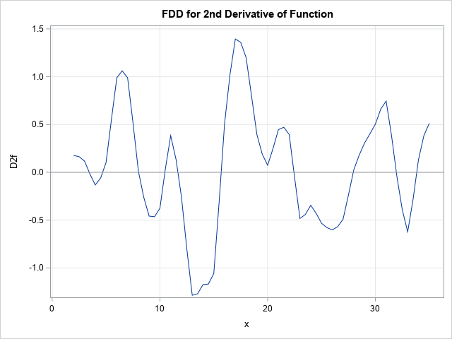
The graph approximates the second derivative for the discrete function. To find the inflection points, we need to locate the locations where the second derivative function crosses the X axis. From the graph, you can estimate that the second derivative is zero near x = 3, 5, 8, 11, and so forth. The next section finds these locations more accurately.

The roots of a discrete function

Since we know the second derivative function only at a discrete set of points, let's approximate the unknown function by a piecewise linear function that "connects the dots" in the graph. We want to find the places where this piecewise linear function crosses the X axis. As explained in a previous article, you can use the DIF function to discover where a function changes sign from positive to negative or vice versa. Consequently, the following PROC IML statements detect where a function changes sign:

/* find where the function changes sign */
dif = dif(f >= 0);
i = T( loc( f^=. & dif^=0 ) );
print i (x[i])[L='x'] (f[i])[L='2nd Deriv']  (dif[i])[L='dif'];

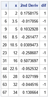
The table shows the values of i for which f[i-1] and f[i] have different signs. When the DIF value is -1, the function is changing from positive to negative. When the DIF value is +1, the function is changing from negative to positive. With this information, you can easily extract the intervals on which the function changes sign. The intervals will be of the form [xL, xR] and the corresponding function values are fL and fR.

/* find intervals on which the f vector changes signs */
xL = x[i - 1];
xR = x[i];
fL = f[i - 1];
fR = f[i];
print xL xR fL fR;

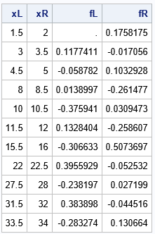
The first point is a "false positive" because the f vector changed from a missing value to a positive value. By using the information in this table and some high-school algebra, you can find the location at which the linear interpolation function is zero:

/* use linear interpolation to estimate the root */
m = (fR - fL) / (xR - xL);     /* slope */
xInflect = xL - fL / m;        /* use point-slope formula to find value of x where f=0 */
print xInflect;

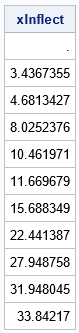
If you prefer to visualize the inflection points on the original graph of the function, you can solve for the corresponding y values and overlay the inflection points on the graph of the function itself, as follows:

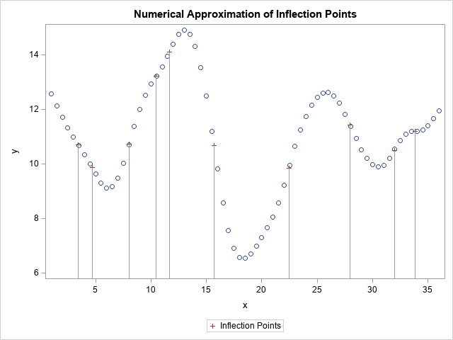
Some of the inflection points might not persist if you jitter some of the data values or slightly modify the smoothing parameter in the thin-plate spline. For example, the points at x=4.68, 10.46, and 11.67 might vanish if the smoothing parameter changes. The other inflection points seem more robust to small changes in the model.

Summary

In summary, this article shows how to approximate the location of inflection points for a function that is known only at a finite set of points. This situation occurs often in statistics. For example, nonparametric regression curve and nonparametric density estimate do not have explicit formulas. Nevertheless, you can use techniques from numerical analysis to approximate the second derivative function. You can then use a cool trick (the DIF function) to detect and approximate the roots of the second derivative function.

For your convenience, the Appendix encapsulates the root-fining statements into a SAS IML function and demonstrates how to solve the problem by using only two function calls.

Appendix

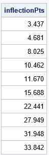
The following SAS IML program approximates the inflection points of a function that is known only at a finite set of points.

proc iml;
/* finite-difference approximation of the second derivative for a 
   function that is known only at discrete points (x[i], y[i]) */
start FDD2(x, y);
   h = dif(x);
   ym2 = lag(y, -2);
   ym1 = lag(y, -1);
   yp1 = lag(y,  1);
   yp2 = lag(y,  2);
   *D1f = (yp1 - ym1) / (2*h);
   D2f = (-yp2 + 16*yp1 - 30*y + 16*ym1 - ym2) / 
         (12*h##2);
   return( D2f );
finish;
 
/* given a function at the points (x[i], y[i]), use linear interpolation
   to find the approximate roots of the function */
start FindDiscreteRoots(x, y);
   dif = dif(y >= 0);
   idx = T( loc( y^=. & dif^=0 ) );
   /* find intervals on which the y vector changes signs */
   xL = x[idx - 1];
   xR = x[idx];
   yL = y[idx - 1];
   yR = y[idx];
   /* use linear interpolation to improve the estimate of the root */
   m = (yR - yL) / (xR - xL);
   roots = xL - yL / m;
   /* if there are any missing values, remove them */
   jdx = loc(roots^=.);
   return( roots[jdx] );
finish;
 
use InData;
read all var {'x' 'y'};
close;
 
f = FDD2(x, y);
inflectionPts = FindDiscreteRoots(x, f);
print  inflectionPts[F=bestd7.];