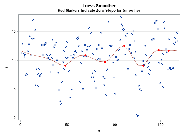
This article shows how to find local maxima and maxima on a regression curve, which means finding points where the slope of the curve is zero. An example appears at the right, which shows locations where the loess smoother in a scatter plot has local minima and maxima. Except for simple cases like quadratic regression, you need to use numerical techniques to locate these values.

In a previous article, I showed how to use SAS to evaluate the slope of a regression curve at specific points. The present article applies that technique by scoring the regression curve on a fine grid of point. You can use finite differences to approximate the slope of the curve at each point on the grid. You can then estimate the locations where the slope is zero.

In this article, I use the LOESS procedure to demonstrate the technique, but the method applies equally well to any one-dimensional regression curve. There are several ways to score a regression model:

• Most parametric regression procedures in SAS (GLM, GLIMMIX, MIXED, ...) support the STORE statement. The STORE statement saves a representation of the model in a SAS item store. You can use PROC PLM to score a model from an item store.
• Some nonparametric regression procedures in SAS do not support the STORE statement but support a SCORE statement. PROC ADAPTIVEREG and PROC LOESS are two examples. This article shows how to use the SCORE statement to find points where the regression curve has zero slope.
• Some regression procedures in SAS do not support either the STORE or SCORE statements. For those procedures, you need to use the use the missing value trick to score the model.

The technique in this article will not detect inflection points. An inflection point is a location where the curve has zero slope but is not a local min or max. Consequently, this article is really about "how to find a point where a regression curve has a local extremum," but I will use the slightly inaccurate phrase "find points where the slope is zero."

How to find locations where the slope of the curve is zero?

For convenience, I assume the explanatory variable is named X and the response variable is named Y. The goal is to find locations where a nonparametric curve (x, f(x)) has zero slopes, where f(x) is the regression model. The general outline follows:

1. Create a grid of points in the range of the explanatory variable. The grid does not have to be evenly spaced, but it is in this example.
2. Score the model at the grid locations.
3. Use finite differencing to approximate the slope of the regression curve at the grid points. If the slope changes sign between consecutive grid points, estimate the location between the grid points where the slope is exactly zero. Use linear interpolation to approximate the response at that location.
4. Optionally, graph the original data, the regression curve, and the point along the curve where the slope is zero.

Example data

SAS distributes the ENSO data set in the SASHelp library. You can create a DATA step view that renames the explanatory and response variables to X and Y, respectively, so that it is easier to follow the logic of the program:

/* Create VIEW where x is the independent variable and y is the response */
data Have / view=Have;
set Sashelp.Enso(rename=(Month=x Pressure=y));
keep x y;
run;

Create a grid of points

After the data set is created, you can use PROC SQL to find the minimum and maximum values of the explanatory variable. You can create an evenly spaced grid of points for the range of the explanatory variable.

/* Put min and max into macro variables */
proc sql noprint;
  select min(x), max(x) into :min_x, :max_x 
  from Have;
quit;
 
/* Evaluate the model and estimate derivatives at these points */
data Grid;
dx = (&max_x - &min_x)/201;    /* choose the step size wisely */
do x = &min_x to &max_x by dx;   
   output;
end;
drop dx;
run;

Score the model at the grid locations

This is the step that will vary from procedure to procedure. You have to know how to use the procedure to score the regression model on the points in the Grid data set. The LOESS procedure supports a SCORE statement, so the call fits the model and scores the model on the Grid data set:

/* Score the model on the grid */
ods select none;    /* do not display the tables */
proc loess data=Have plots=none;
   model y = x;
   score data=Grid;  /* PROC LOESS does not support an OUT= option */
   /* Most procedures support an OUT= option to save the scored values.
      PROC LOESS displays the scored values in a table, so use ODS to
      save the table to an output data set */
   ods output ScoreResults=ScoreOut;
run;
ods select all;

If a procedure supports the STORE statement, you can use PROC PLM to score the model on the data. The SAS program that accompanies this article includes an example that uses the GAMPL procedure. The GAMPL procedure does not support the STORE or SCORE statements, but you can use the missing value trick to find zero derivatives.

Find the locations where the slope is zero

This is the mathematical portion of the computation. You can use a backward difference scheme to estimate the derivative (slope) of the curve. If (x0, y0) and (x1, y1) are two consecutive points along the curve (in the ScoreOut data set), then the slope at (x1, y1) is approximately m = (y1 - y0) / (x1 - x0). When the slope changes sign between consecutive points, it indicates that the slope changed from positive to negative (or vice versa) between the points. If the slope is continuous, it must have been exactly zero somewhere on the interval. You can use a linear approximation to find the point, t, where the slope is zero. You can then use linear interpolation to approximate the point (t, f(t)) at which the curve is a local min or max.

You can use the following SAS DATA step to process the scoring data, approximate the slope, and estimate where the slope of the curve is zero:

/* 4. Compute slope by using finite difference formula. */
data Deriv0;
set ScoreOut;
Slope = dif(p_y) / dif(x);      /* (f(x) - f(x-dx)) / dx */
/* save previous values of x, y, and slope */
xPrev = lag(x);  yPrev = lag(p_y); SlopePrev = lag(Slope);
if n(SlopePrev) AND sign(SlopePrev) ^= sign(Slope) then do;
   /* The slope changes sign between this obs and the previous.
      Assuming linearity on the interval, find (t, f(t))
      where slope is exactly zero */
   t0 = xPrev - SlopePrev * (x - xPrev)/(Slope - SlopePrev); 
   /* use linear interpolation to find the corresponding y value:
      f(t) ~ y0 + (y1-y0)/(x1-x0) * (t - x0)       */
   f_t0 = yPrev + (yPrev - p_y)/(x - xPrev) * (t0 - xPrev);
   if sign(SlopePrev) > 0 then _Type_ = "Max";
   else _Type_ = "Min";
   output; 
end;
keep t0 f_t0 Slope _Type_;
label f_t0 = "f(t0)";
run;
 
proc print data=Deriv0 label;
run;

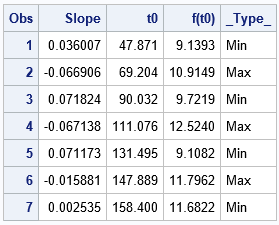
The table shows that there are seven points at which the derivative of the loess regression curve has a local min or max.

Graph the results

If you want to display the local extreme on the graph of the regression curve, you can concatenate the original data, the regression curve, and the local extreme. You can then use PROC SGPLOT to overlay the three layers. The resulting graph is shown at the top of this article.

data Combine;
merge Have                           /* data   : (x, y)     */
      ScoreOut(rename=(x=t p_y=p_t)) /* curve  : (t, p_t)   */
      Deriv0;                        /* extrema: (t0, f_t0) */
run;
 
title "Loess Smoother";
title2 "Red Markers Indicate Zero Slope for Smoother";
proc sgplot data=Combine noautolegend;
   scatter x=x y=y;
   series x=t y=p_t / lineattrs=GraphData2;
   scatter x=t0 y=f_t0 / markerattrs=(symbol=circlefilled color=red);
   yaxis grid; 
run;

Summary

In summary, if you can evaluate a regression curve on a grid of points, you can approximate the slope at each point along the curve. By looking for when the slope changes sign, you can find local minima and maxima. You can then use a simple linear estimator on the interval to estimate where the slope is exactly zero.

You can download the SAS program that performs the computations in this article.