Generate correlation matrices with specified eigenvalues

A previous article discusses how to generate a random covariance matrix with a specified set of (positive) eigenvalues. A SAS programmer asked whether it is possible to produce a correlation matrix that has a specified set of eigenvalues. After discussing the problem with a friend, I am happy to report that, yes, it is possible to implement an iterative algorithm that converges to a random correlation matrix that has a specified set of eigenvalues.

The set of eigenvalues for a matrix is called the spectrum. Thus, this post shows how to construct a random correlation matrix with a given spectrum.

Can we just convert a covariance matrix to a correlation matrix?

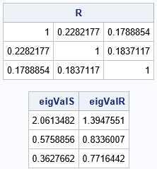
You might hope that we can use the relationship between a covariance matrix and a correlation matrix to solve this problem. Recall that it is easy to rescale a covariance matrix to obtain a unit diagonal. Alas, rescaling a covariance matrix changes the eigenvalues and eigenvectors! This is easily shown by using an example. The following SAS IML program defines a 3 x 3 covariance matrix, S. The program uses the COV2CORR function to obtain the corresponding correlation matrix. It then calls the EIGVAL function compute the eigenvalues for both matrices and displays the results:

proc iml;
/* start with a symmetric positive definite matrix (a covariance matrix) */
S = {2.0   0.25  0.16,
     0.25  0.6   0.09,
     0.16  0.09  0.4};
/* The naive attempt to obtain a correlation matrix is to scale the 
   covariance matrix to get unit diagonals, but that destroys the eigenvalues */
R = cov2corr(S);
eigValS = eigval(S);
eigValR = eigval(R);
print R;
print eigValS eigValR;

Recall that the sum of the eigenvalues of a matrix is equal to the trace of the matrix, which means that the trace of an n x n correlation matrix equals n. For this 3 x 3 example, I intentionally chose the diagonal elements of the original matrix to be 3. Nevertheless, as shown above, converting the covariance matrix to a correlation matrix changes the eigenvalues.

The method of alternating projections

Although the one-step conversion from covariance to correlation matrix does not solve the problem, it can be used in an iterative algorithm known as the method of alternating projections (MAP). I have used MAP in the past to work with correlation matrices. Specifically, I used it to find the nearest correlation matrix to an arbitrary symmetric matrix.

The method of alternating projections is used to find an element in the intersection of two sets. For this problem, the two sets are:

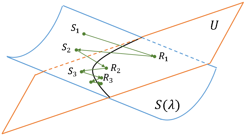
S(λ), which is the set of all SPD covariance matrices that have the spectrum λ = {λ₁, λ₂, ..., λ_n}, where Σ λ_i = n. It is drawn as a blue surface in the illustration at the right.
U, which is the set of all SPD correlation matrices. It is drawn as an orange plane in the illustration at the right.

The MAP algorithm starts with a guess in one of the sets, such as the point S₁ in S(λ). You then "project" or otherwise convert the guess to a point in the other set, such as R₁ in U. You then transform the point back to the first set S(λ). By repeating these transformations, you hope the iteration converges to the intersection of the two sets, which will be a correlation matrix with the specified spectrum.

When the sets are convex, you can show that MAP converges to an element in the intersection (Dykstra, 1983, JASA). In this problem, the set of correlation matrices is convex, but, unfortunately, the set of SPD matrices that have the same spectrum is not convex. However, Lewis, Luke, and Malick (2009) showed that MAP can achieve local convergence when only one set is convex. Thus, we can implement MAP and hope that it works in practice.

That is what Waller (2020, TAS) did. Based on a simulation study, he reported that the MAP converged for every simulated spectrum that he used. The following MAP algorithm is slightly modified from Waller (2020):

Choose a spectrum for the correlation matrix. Define the spectrum as λ = {λ₁, λ₂, ..., λ_n}, where Σ λ_i = n
Create a random covariance matrix, S₁, that has the desired spectrum. The link shows how to implement this step in SAS.
Convert the covariance matrix to a correlation matrix, R. I suggest scaling the covariance matrix by using the COV2CORR function in SAS IML software. This ensures that you obtain a true SPD correlation matrix.
If R has the desired eigenvalues within some tolerance, the problem is solved. Otherwise, use the eigenstructure of R to create a new covariance matrix that has the same eigenvectors but the desired spectrum. Specifically, if the spectral decomposition of R is Q*D*Q`, define the new covariance matrix as Q*diag(λ)*Q`.
Iterate Steps 3 and 4 until convergence.

Choose a random covariance matrices that has the specified eigenvalues

Let's review how to construct a random covariance matrix with a specific spectrum. Recall that a covariance matrix is symmetric and positive definite, which means that all its eigenvalues are positive. Next, recall the Spectral Decomposition Theorem for symmetric matrices, which states that every symmetric matrix, A, can be decomposed as the product A = Q*D*Q` where Q is an orthogonal matrix whose columns are the eigenvectors of A and where D is a diagonal matrix that contains the corresponding eigenvalues of A. The spectral decomposition is also called the eigendecomposition of A.

In linear algebra, you typically start with the symmetric matrix A, and you calculate the eigenvalues and vectors to obtain the matrices D and Q. However, as I showed previously, you can go the other direction. If you start with a set of positive eigenvalues (D) and generate a random orthogonal matrix, Q, then the matrix Q*D*Q` is, by construction, a symmetric matrix that has a positive spectrum. Consequently, it is a covariance matrix.

My previous article about how to generate a random orthogonal matrix uses an algorithm (Stewart, 1980) that produces uniformly distributed matrices in the space of orthogonal matrices. Thus, if you repeat the MAP algorithm many times in a simulation study, you are likely to produce a wide range of Q matrices and therefore sample uniformly from the set S(λ). Be aware that some authors use initial matrices that are not uniformly distributed.

Convert a covariance matrix to a correlation matrix

In Waller's implementation of MAP, he projects each a covariance matrix onto the space of matrices that have 1s on their main diagonal. (I used the same transformation in my previous implementation of MAP.) For the current problem, I think it is better to scale the covariance matrix to form a real correlation matrix. Why? Because setting the diagonal elements to 1 can result in a matrix that is not positive definite. It seems useful to ensure that the MAP algorithm is using an SPD matrix at every step.

Implement the method of alternating projections in SAS

The Appendix defines the SAS IML algorithm that implements the method of alternating projections. I created multiple helper functions so that each step of the algorithm has its won function. The main function (CorrWithEigen) takes a vector of n eigenvalues (the spectrum) as the required argument. If the sum of the eigenvalues does not equal n, the vector is rescaled. The algorithm then creates a random initial covariance matrix that has the specified eigenvalues, and alternates projecting the matrices onto U (the set of correlation matrices) and S(λ) (the set of SPD covariance matrices that have the spectrum) until it converges to a correlation matrix that has the spectrum. The details are in the Appendix.

The following program loads CorrWithEigen function and run the algorithm for the spectrum λ = {3, 0.5, 0.3, 0.2}.

proc iml;
load module=_all_;   /* modules are defined in the Appendix */
call randseed(1234, 1);
Spectrum = {3, 0.5, 0.3, 0.2};
 
/* call the MAP algorithm multiple times */
R1 = CorrWithEigen(Spectrum);
R2 = CorrWithEigen(Spectrum);
R3 = CorrWithEigen(Spectrum);
 
/* verify that each correlation matrix has the required spectrum */
eigR1 = eigval(R1);
eigR2 = eigval(R2);
eigR3 = eigval(R3);
print Spectrum eigR1 eigR2 eigR3;
/* the spectrum is the same, but the correlations are different */
labl = 'X1':'X4';
print R1[r=labl c=labl], R2[r=labl c=labl], R3[r=labl c=labl];

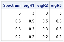
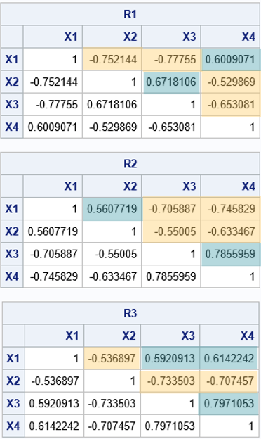
The first table in the output shows that each correlation matrix has the required spectrum (within some convergence criterion). The next tables print the correlation matrices. I have overlaid colors to emphasize which pairs of correlations are positive and which are negative. Notice that the spectrum does NOT determine the correlations! There are several different correlation matrices that have the same spectrum. For the three in this example:

For the R1 correlation matrix, the positive correlations are Corr(X1, X4) and Corr(X2, X3).
For the R2 correlation matrix, the positive correlations are Corr(X1, X2) and Corr(X3, X4).
For the R3 correlation matrix, the positive correlations are Corr(X1, X3), Corr(X1, X4), and Corr(X3, X4).

There is much more that can be said about the distribution of the elements for the correlation matrix, but that discussion will have to wait for another article.

Random versus arbitrary

This algorithm generates a set of different correlation matrices, all with the same spectrum. However, I do not know the probability distribution of the correlation matrices that result from this algorithm. It might be that some correlation matrices are more probable than others.

Summary

A previous article discusses how to generate a random covariance matrix with a specified set of (positive) eigenvalues. This article shows how to produce a correlation matrix that has a specified set of eigenvalues. The eigenvalues must sum to n, where n is the dimension of the matrix. The Appendix provides SAS IML functions to generate correlation matrices from a specified spectrum by using the method of alternating projections (Waller, 2020)

Appendix: SAS program for generating correlation matrices with specified eigenvalues

The following SAS IML program uses the method of alternating projections (MAP) to generate an arbitrary correlation matrix that has a specified set of eigenvalues (spectrum). The program is similar to the algorithm proposed by Waller (2020, TAS), except for the following steps:

To get the initial guess, Waller generates an orthogonal matrix, Q, by using the QR decomposition of a matrix that has normal random variates. I use Stewart's algorithm (Stewart, 1980) to produces uniformly distributed orthogonal matrices.
I project each covariance matrix onto the space of correlation matrices. Waller projects onto the space of symmetric matrices with unit diagonal, which might not be positive definite.

/* SAS code to accompany "Generate correlation matrices with specified eigenvalues"
by Rick Wicklin. Published on The DO Loop blog on 18DEC2024.
https://blogs.sas.com/content/iml/2024/12/18/correlation-matrix-eigenvalues.html
 
Use the method of alternating projections (MAP) to find a correlation 
matrix that has a specified spectrum (eigenvalues). The projections are:
1. Choose a spectrum Lambda = {L1, L2, ..., Ln} where L_i>0 and sum(Lambda)=n.
2. Create a covariance matrix, S, that has the specified eigenvalues.
3. Convert the matrix to a correlation matrix, R.
4. If R has the desired eigenvalues, quit. Otherwise,
   use the eigenstructure of R to create a new covariance matrix that has
   the same eigenvectors but the desired eigenvalues. Go to Step 3.
 
I have previously use MAP to find the nearest correlation matrix:
https://blogs.sas.com/content/iml/2012/11/28/computing-the-nearest-correlation-matrix.html
This implementation of MAP uses similar functions:
Given a spectrum L={L1, L2, ..., LN} start with a random SPD
matrix Q*diag(L)*Q` where Q is an arbitrary orthogonal matrix.
Then use 
ProjU: project a covariance matrix, S, onto U={correlation matrix for S}
ProjS: project a correlation matrix onto 
       S(lambda)={positive semidefinite matrices that has spectrum L}
*/
proc iml;
/* To get a random orthogonal matrix, use 
   https://blogs.sas.com/content/iml/2012/03/28/generating-a-random-orthogonal-matrix.html
   To get a random SPD matrix, use 
   https://blogs.sas.com/content/iml/2012/03/30/geneate-a-random-matrix-with-specified-eigenvalues.html
*/
/* Generate random orthogonal matrix G. W. Stewart (1980).    
   Algorithm adapted from QMULT MATLAB routine by Higham (1991) */
start RndOrthog(n);
A = I(n);
d = j(n,1,0);
d[n] = sgn(RndNormal(1,1));
do k = n-1 to 1 by -1; 
   /* generate random Householder transformation */
   x = RndNormal(n-k+1,1);
   s = sqrt(x[##]); /* norm(x) */
   sgn = sgn( x[1] );
   s = sgn*s;
   d[k] = -sgn;
   x[1] = x[1] + s;
   beta = s*x[1];
   /* apply the transformation to A */
   y = x`*A[k:n, ];
   A[k:n, ] = A[k:n, ] - x*(y/beta);
end;
A = d # A; /* change signs of i_th row when d[i]=-1 */
return(A);
finish;
 
/**** Helper functions ****/
/* Compute SGN(A). Return matrix of same size as A with 
   m[i,j]= {  1 if A[i,j]>=0
           { -1 if A[i,j]< 0           */
start sgn(A);
return( choose(A>=0, 1, -1) );
finish;
 
/* return (r x c) matrix with standard normal variates */
start RndNormal(r,c);
   x = j(r,c);
   call randgen(x, "Normal");
   return(x);
finish;
 
start RndMatWithEigenval(_lambda);
   lambda = rowvec(_lambda);   /* ensure lambda is row vector */
   n = ncol(lambda);
   Q = RndOrthog(n);
   return( Q`*diag(lambda)*Q ); 
finish;
 
/* efficient computation of A*D*A` where D = diag(v) and v[i]>0 for all i */
start QuadFormDiagPos(A, v);
   D = rowvec(v);     /* ensure D is row vector */
   W = A#sqrt(D);     /* left half of A*diag(v)*A` */
   return( W*W` );    /* W*W` = A*diag(v)*A` */
finish;
 
/* Project symmetric A onto S = {positive semidefinite matrices} */
start ProjS(A, lambda);
   call eigen(D, Q, A);             /* A = Q*D*Q` */
   S = QuadFormDiagPos(Q, lambda);  /* S = Q*diag(lambda)*Q` */
   return S;
finish;
 
/* project SPD matrix S onto U={correlation matrices}.
   Return correlation matrix for S. */
start ProjU(S);
   return cov2corr(S);
finish;
 
/* Helper function: the L2 norm of the difference between 
   targetLambda and the eigenvalues of a symmetric matrix A.
   Assume targetLambda is sorted from largest to smallest. */
start DistBetweenEigenvalues(A, targetLambda);
   lambda = eigval(A);
   return( sqrt(SSQ(targetLambda - lambda)) );
finish;
 
/* for column vector v, standardize so sum(v)=nrow(v) */
start StdizeEigenval(v);
    L = colvec(v);
    return ( L * nrow(L)/sum(L) );  /* make sum(v)=dimension */
finish;
 
/* Encapsulate the MAP algorithm into a function */
start CorrWithEigen(targetLambda, tol=1e-10, maxIters=500);
   lambda = StdizeEigenval(targetLambda);
   /* generate a random orthogonal matrix and use to construct PSD matrix with spectrum */
   S = RndMatWithEigenval(lambda); /* eigenvalues are lambda */
   delta = 1E6;
   do k = 1 to maxIters while(delta > tol);
      /* project onto space of correlation matrices (or matrices with unit diagonal) */
      R = ProjU(S);
      /* project R onto matrices with the spectrum */
      S = ProjS(R, lambda);
      delta = DistBetweenEigenvalues(R, lambda);
   end;
   R = ProjU(S);   /* final projection */
   return R;
finish;
store module = _all_;
QUIT;
 
/* Example: load the modules and use them to generate correlation matrices with specified spectrum */
proc iml;
load module=_all_;   /* modules are defined in the Appendix */
call randseed(1234);
Spectrum = {3, 0.5, 0.3, 0.2};
 
/* call the MAP algorithm multiple times */
R1 = CorrWithEigen(Spectrum);
R2 = CorrWithEigen(Spectrum);
R3 = CorrWithEigen(Spectrum);
 
/* verify that each correlation matrix has the required spectrum */
eigR1 = eigval(R1);
eigR2 = eigval(R2);
eigR3 = eigval(R3);
print Spectrum eigR1 eigR2 eigR3;
/* the spectrum is the same, but the correlations are different */
labl = 'X1':'X4';
print R1[r=labl c=labl], R2[r=labl c=labl], R3[r=labl c=labl];

Blogs