A colleague asked me an interesting question: Suppose you have a structured correlation matrix, such as a matrix that has a compound symmetric, banded, or an AR1(ρ) structure. If you generate a random correlation matrix that has the same eigenvalues as the structured matrix, does the random matrix have the same structure?
The answer is no. The common structures used by statistical modelers are not preserved. However, there is a different kind of "structure" in the cells of the random matrices. This article provides a complete analysis of 2 x 2 and 3 x 3 correlation matrices that have a common spectrum. The 3 x 3 example reveals many characteristics of the general d x d case.
Recall that the spectrum for a matrix is the set of eigenvalues. The following facts are used in this article:
- For any matrix, the sum of the eigenvalues equals the trace of the matrix. Because a correlation matrix has 1s on the diagonal, the eigenvalues of a d x d correlation matrix must sum to d.
- The eigenvalues of a correlation matrix are nonnegative.
- Thus, for a correlation matrix, the spectrum is an element of the simplex defined by Σ λi = d and λi ≥ 0.
Two-dimensional correlation matrices
In the 2 x 2 case, every correlation matrix is a symmetric matrix that has 1s on the diagonal and a number ρ for the two off-diagonal elements, where -1 ≤ ρ ≤ 1. Assume that we are given a 2 x 2 correlation matrix, A, that has a specified spectrum Λ = {λ1, λ2}. What does A look like?
As shown in a previous article, the squared Frobenius norm of a symmetric matrix always equals the sum of the squared eigenvalues. The squared Frobenius norm is || A ||2 = 2 + 2*ρ2. Therefore, every matrix that has the same spectrum also has this Frobenius norm.
By using this fact, we can characterize all 2 x 2 matrices that have a specific spectrum. Let R2 be the sum of the squared eigenvalues. From the formula for || A ||2, we know that ρ2 = (R2 – 2)/2. (Note that R2 ≥ 2.) Consequently, there are exactly two correlation matrices that have the same spectrum: one where ρ is the positive square root of (R2 – 2)/2, and one where ρ is the negative of the square root.
In summary, we know the form of all 2 x 2 correlation matrices that have the spectrum Λ. You compute R2, which is the sum of the squared eigenvalues. Then, the correlation matrices have the value ρ or -ρ on the off-diagonal, where ρ2 = (R2 - 2)/2.
The geometry of 2-D correlation matrices
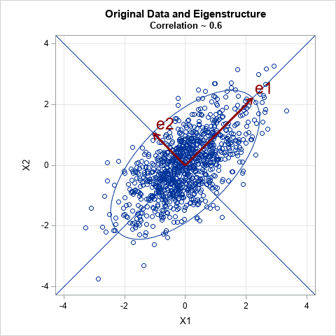
One interpretation of a correlation matrix is as the association between two bivariate normal continuous variables that have been standardized to have mean 0 and unit standard deviation. The following image shows a scatter plot for 1,000 observations for two variables X1 and X2, whose correlation is 0.6. The spectrum is {1 ± ρ} = {1.6, 0.4}. For eigenvectors, you can choose e1={1,1} and e2={-1,1}. When scaled appropriately, the eigenvectors equal the semi-major and semi-minor axes of the probability ellipse for the data.

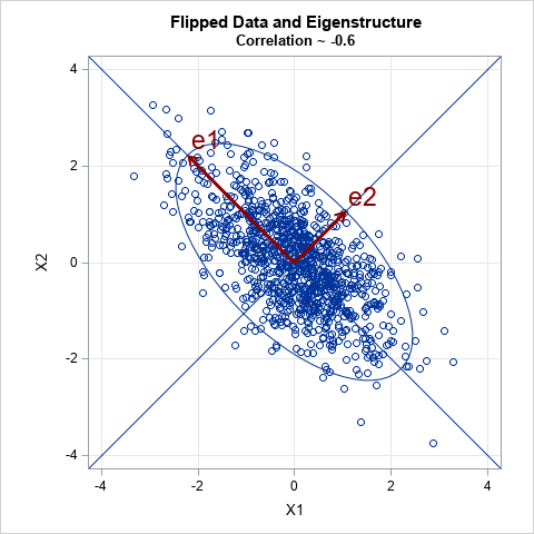
We've shown that another correlation matrix that has the same spectrum is the matrix with -0.6 as the off-diagonal element. Geometrically, you can think of this matrix as the correlations between the variables –X1 and X2. That is, if you multiply one of the variables by –1, you reverse the sign of the correlation. The following image shows the geometry for this second case:

If you think of the spectrum of a correlation matrix as representing the geometry of a probability ellipse of centered data, then it is clear that reflections across any axis do not change the geometry. For centered data, a geometric refection is the same as multiplying a variable by –1. From this geometric perspective, it is clear that we can always find a new matrix that has the same spectrum simply by changing the sign of all off-diagonal elements in a chosen row and column. In the 2 x 2 correlation matrix, we can always change the sign of the off-diagonal elements in the first row and column, or in the second row and column. (Because a correlation matrix is symmetric, the two operations are the same.)
3 x 3 correlation matrices
A general 3 x 3 correlation matrix, A, has three parameters for the off-diagonal elements in the upper-triangular portion of A. (By symmetry, these cells are the same as the cells in the lower-triangular portion of A.) If you change the sign of any underlying variable, you obtain a different correlation matrix that has the same spectrum. That is, if (R12, R13, R23) are the off-diagonal elements of A, then the eigenvalues are unchanged for the following matrices:
- Change the sign of X1, which means that the off-diagonal elements of the correlation matrix are (-R12, -R13, R23)
- Change the sign of X2, which results in the off-diagonal elements (-R12, R13, -R23)
- Change the sign of X3, which results in the off-diagonal elements (R12, -R13, -R23)
Are these the only matrices that have the same spectrum? No! To see some other matrices, let's run a numerical example. Let's start with a correlation matrix that has an AR1(ρ=0.5) structure. The off-diagonal elements for this matrix are (R12, R13, R23) = (0.5, 0.25, 0.5). The spectrum of this matrix is {1.843, 0.75, 0.407}. Let's use the modules from a previous article to generate 5,000 correlation matrices that have this spectrum and plot the values of the three off-diagonal cells (R12, R13, R23):
/* Visualize the off-diagonal elements for a 3x3 correlation matrix that has the same spectrum as an AR1(rho) matrix */ proc iml; /* modules are defined in the Appendix at https://blogs.sas.com/content/iml/2024/12/18/correlation-matrix-eigenvalues.html */ load module=_all_; call randseed(12345); /* AR1 correlation structure: https://blogs.sas.com/content/iml/2012/11/05/constructing-common-covariance-structures.html */ Sigma = {1.0 0.5 0.25, 0.5 1.0 0.5, 0.25 0.5 1.0}; Spectrum = eigval(Sigma); /* approx {1.843, 0.75, 0.407} */ NSim = 5000; /* simulate NSim random matrices */ result = j(NSim, 3); do i = 1 to NSim; R = CorrWithEigen(Spectrum); result[i,] = rowvec( R[{2 3 6}] ); /* save the off-diagonal values */ end; /* write the off-diagonal values to a data set */ create RSim from result[c={R12 R13 R23}]; append from result; close; QUIT; title "Cell Values for 3x3 Matrices That Have a Common Spectrum"; proc sgplot data=RSim2 aspect=1; scatter x=R12 y=R13 / markerattrs=(symbol=CircleFilled size=3) colorresponse=R23; refline 0 /axis=x; refline 0 /axis=y; xaxis grid; yaxis grid; run; |

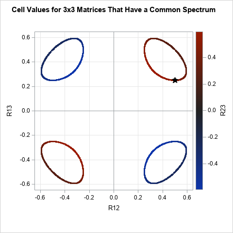
The graph shows the R12 and R13 values for 5,000 correlation matrices that have the spectrum {1.843, 0.75, 0.407}. The color indicates the value of the R23 cell. The closed curve in the upper-right quadrant is reflected across the horizontal and vertical axes to create the other curves. You can see that the R23 value is positive when R12 and R13 have the same sign and is negative otherwise. The star-shaped marker indicates the off-diagonal values for the original AR1(ρ=0.5) matrix.
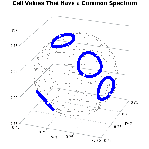
Of course, this graph is actually the projection onto the (R12, R13)-plane of three-dimensional points (R12, R13, R23). From the color of the markers, we know that the points in the first and third quadrants are high in the R23 direction whereas the points in the second and fourth quadrants are low in R23. But we know more than that! Because every point represents a matrix, and because the Frobenius norm of these matrices are the same, we know that the (R12, R13, R23) values satisfy the equation R122 + R132 + R232 = S2, where S2 = (R2 - 3)/2 and R2 is the sum of the squared eigenvalues. Thus, these points lie on the surface of a sphere with radius S = 0.75. You can use PROC G3D in SAS to plot the points and the outline of a 3-D sphere:

Voilà! This is the visualization of the set of 3 x 3 correlation matrices that have the spectrum {1.843, 0.75, 0.407}. The graph shows the possible values of the off-diagonal elements (R12, R13, R23). The points are constrained to lie on the surface of a sphere with radius 0.75.
Other matrices on the sphere
Every point on the sphere represents a 3 x 3 correlation matrix, so you might wonder about the other matrices on the sphere. They correspond to matrices that have different spectra but the same matrix norm. For example, here are some other points on the sphere:
- The point (0, 0, 0.75) is the "north pole" of the sphere. The correlation matrix with those off-diagonal values has the spectrum {1.75, 1, 0.25}, which is different from the spectrum of the AR1(ρ=0.5) matrix. However, both spectra have the same vector norm.
- The point (0.4, 0.492, 0.4) is on the sphere and represents a Toeplitz (banded) matrix. Its spectrum is {1.863, 0.629, 0.508}, which also has the same vector norm.
So, the sphere can be decomposed into a fibration for a family of curves. Each curve corresponds to a 3-element spectrum, Λ, such that || Λ ||2 = 4.125. For most values of || Λ ||, there are four connected curves, as explained earlier.
Higher-dimensional correlation matrices
Some of the previous ideas generalize to higher dimensions:
- The Frobenius norm of a correlation matrix equals the vector norm of its spectrum, thought of as a vector. Since the diagonal elements are 1, the off-diagonal elements of a d x d correlation matrix must lie on a sphere Σ Rij2 = R2, where R2 = (|| Λ ||2 - d) / 2 and the sum is over cells i < j.
- The sphere is k-dimensional where k = d*(d – 1)/2. The sphere decomposes into disjoint sets. Within each set, all matrices have a Frobenius norm equal to the norm of the spectrum.
Summary
Let A be a d-dimensional correlation matrix that has the spectrum Λ = {λ1, λ2, ..., λd}, where Σ λi = d and all λi ≥ 0. The off-diagonal elements of A lie on a sphere of radius R, where R2 = (|| Λ ||2 - d) / 2 and the sum is over cells i > j. This article uses geometry, linear algebra, and functional analysis to visualize the set of correlation matrices that have a common spectrum.
You can download the SAS program that creates all graphs in this article:
