Because I am writing a new book about simulating data in SAS, I have been doing a lot of reading and research about how to simulate various quantities. Random integers? Check! Random univariate samples? Check! Random multivariate samples? Check!
Recently I've been researching how to generate random matrices. I've blogged about random matrices before, when I noted that the chance of encountering a singular matrix "at random" is zero. I am mostly interested in generating random correlation (or covariance) matrices because these matrices are useful in statistical simulation, but I've also encountered journal articles about generating other kinds of matrices. In this article I show how to generate a random orthogonal matrix and show that the distribution of eigenvalues of these matrices is very interesting.
Orthogonal matrices
An orthogonal matrix is a matrix Q such that Q`Q=I. The determinant of an orthogonal matrix is either 1 or –1. Geometrically, an othogonal matrix is a rotation, a reflection, or a composition of the two.
G. Stewart (1980) developed an algorithm that generates random orthogonal matrices from the Haar distribution. Although "Haar distribution" might sound scary, it just means that the matrices are generated uniformly in the space if orthogonal matrices. In that sense, that algorithm is like picking a number with a probability that is uniform in [0,1].
Although I usually blog about how to implement algorithms efficiently in the SAS/IML language, today I'm just going to present the SAS/IML program in it's final form and direct you to Stewart's paper for the details and description of why it works. The algorithm can be summarized by saying that random normal variates are used to fill up rows of a matrix, and Householder transformations are used to induce orthogonality. The algorithm is presented below:
proc iml;
/* Generate random orthogonal matrix G. W. Stewart (1980).
   Algorithm adapted from QMULT MATLAB routine by Higham (1991) */
start RndOrthog(n);
A = I(n);
d = j(n,1,0);
d[n] = sgn(RndNormal(1,1));
do k = n-1 to 1 by -1;
   /* generate random Householder transformation */
   x = RndNormal(n-k+1,1);
   s = sqrt(x[##]); /* norm(x) */
   sgn = sgn( x[1] );
   s = sgn*s;
   d[k] = -sgn;
   x[1] = x[1] + s;
   beta = s*x[1];
   /* apply the transformation to A */
   y = x`*A[k:n, ];
   A[k:n, ] = A[k:n, ] - x*(y/beta);
end;
A = d # A; /* change signs of i_th row when d[i]=-1 */
return(A);
finish;

/**** Helper functions ****/
/* Compute SGN(A). Return matrix of same size as A with
   m[i,j]= {  1 if A[i,j]>=0
           { -1 if A[i,j]< 0           */
start sgn(A);
return( choose(A>=0, 1, -1) );
finish;

/* return (r x c) matrix with standard normal variates */
start RndNormal(r,c);
   x = j(r,c);
   call randgen(x, "Normal");
   return(x);
finish; |
Calling the function
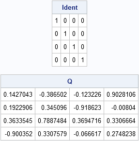
Whenever I program a new function, I immediately check to see if it makes sense. For this function, I will generate a 4x4 matrix and check that Q`Q=I:
call randseed(1); Q=RndOrthog(4); reset fuzz; Ident = Q`*Q; print Ident, Q; |
Eigenvalues of a random orthogonal matrix
Physicists and mathematicians study the eigenvalues of random matrices and there is a whole subfield of mathematics called random matrix theory. I don't know much about either of these areas, but I will show the results of two computer experiments in which I visualize the distribution of the eigenvalues of random orthogonal matrices.
The first experiment is to generate 100 2x2 matrices and plot the 200 eigenvalues. This is done with the following program:N = 200;
evals = j(N, 2, 0); /* 2*N complex values */
p = 2;
do i = 1 to N by p;
e = eigval( RndOrthog(p) );
evals[i:i+p-1, 1:ncol(e)] = e;
end;
create C2 from evals[c={"x" "y"}]; append from evals; close; |
Similarly, I can compute the 200 eigenvalues from a single 200x200 orthogonal matrix, as follows:
/* eigenvalues of 1 200x200 matrix */
evals = eigval( RndOrthog(N) );
create C200 from evals[c={"x" "y"}]; append from evals; close; |
If I plot the distribution of eigenvalues in each case, I get two very different results. Click to see the full sized image:
proc kde data=c2; /* Eigenvalues of 100 2x2 Matrices */ bivar x y / plots=ContourScatter bwm=0.5; run; proc kde data=c200; /* Eigenvalues of 200x200 Matrix */ bivar x y / plots=ContourScatter bwm=0.5; run; |
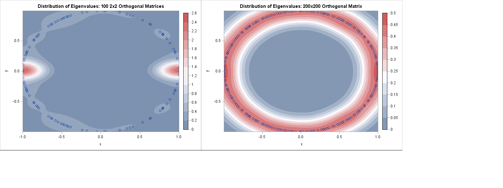
An orthogonal transformation is composed two kinds of "elementary" transformations: reflections and rotations. The distribution of the eigenvalues of the 2x2 matrices shows that about half of the random 2x2 orthogonal matrices are reflections (eigenvalues 1 and -1) and about half are rotations (complex conjugate eigenvalues). I find this interesting because I did not previously know the answer to the question, "what is the distribution of reflections and rotations among 2x2 orthogonal matrices?"
In contrast, for the large 200x200 matrix, the eigenvalues are spread uniformly at random on the unit circle. This is a consequence of a theorem that says as the size of an orthogonal matrix increases, the distribution of the eigenvalues converges to the uniform distribution on the unit circle. (This was noted by Persi Diaconis in his article "What is a Random Matrix.")
If this result is interesting to you, I encourage you to run some computer experiments. I computed the distribution of eigenvalues for random matrices of size 4, 8, 20, 25, and 50, and it is interesting to watch the eigenvalues spread out and become more uniform as the matrix size increases. (I avoided matrices of odd dimension; They always have a real eigenvalue of 1 or -1 because eigenvalues of a real matrix appear in conjugate pairs.) I think it would be fun to watch an animation of the eigenvalues spread out as the dimension of the matrices increase!

2 Comments
Pingback: Geneate a random matrix with specified eigenvalues - The DO Loop
Pingback: The curious case of random eigenvalues - The DO Loop