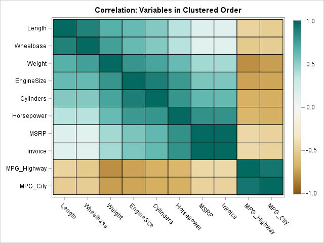
A common way to visualize the sample correlations between many numeric variables is to display a heat map that shows the Pearson correlation for each pair of variables, as shown in the image to the right. The correlation is a number in the range [-1, 1], where -1 indicated perfect negative correlation and +1 indicates perfect positive correlation.

There are alternative methods to visualize the correlation between variables. Several methods use the fact that the correlation coefficient can be understood as the cosine of the angle between vectors. This article shows how to use SAS to create two popular visualizations of the angles between vectors. One method (the loading plot) has been in SAS for decades. A related method (sometimes called the correlogram) is not, to my knowledge, produced by any SAS procedure. However, the correlogram can be obtained by using a nonlinear optimization to find angles for vectors that best fit the sample correlation matrix. This article shows how to run the optimization in PROC IML.

The loadings plot

In factor analysis (which includes principal component analysis), you are often interested in finding a low-dimensional subspace that explains the data well. The word "well" has various meanings, but for principal component analysis the subspace explains a lot of the variance in the data. After you find this subspace, you can project the (standardized) data vectors onto the subspace. The resulting plot is called a loading plot. Vectors that have almost unit length are almost in the subspace; vectors that have a very short length are almost orthogonal to the subspace.

In SAS, you can use PROC FACTOR to create a loading plot, as follows:

%let DSName = Sashelp.Cars;
%let varNames = _NUMERIC_;
proc factor data=&DSName method=principal N=2 /* N= specifies number of factors */
     plots=(scree initloadings(vector));
   var &varNames;
   ods select InitPatternPlot;
run;

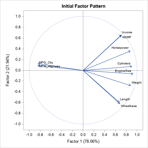
For the Sashelp.Cars data, there are 10 numeric variables, which you can think of as vectors. For each pair of variables, the cosine of the angles between the vectors is equal to the correlation between the variables. However, the loading plot shown above is the projection of the vectors onto the span of two factors. The projected vectors do not have the same angles between them as the unprojected vectors. However, if the two factors explain the data "well," then the angles between the vectors in the loading plot are not too different from the true angles. Consequently, the cosine of the angles between vectors in the loading plot is approximately equal to the correlation between variables.

If the first two factors explain the data well, you can examine the loadings plot and use the angles between vectors to interpret the correlation between variables. In the loading plot shown above, you can observe the following facts:

• Three pairs of variables are highly correlated: The MPG_City and MPG_Highway variables, the Invoice and MSRP variables, and the Length and Wheelbase variables. You can see that the vectors are almost identical.
• The MPG_City and MPG_Highway variables are negatively correlated with the other variables because the vectors point in the opposite direction. variables.
• For any variable, you can read off which other variables are strongly correlated to it. For example, find the vector for the Cylinders variable. The vector that is closest to it is the EngineSize variable. The next closest vectors are Horsepower and Weight. This means that the correlation with the Cylinders variable is highest for EngineSize, followed by Horsepower and Weight.
• The Length (and Wheelbase) variable is almost perpendicular to the Invoice (and MSRP) variable. Therefore, the correlation must be almost zero.

I like the loadings plot because you can use the angles between the vectors to deduce which variables are strongly and weakly correlated with each other. But the loadings plot carries a lot of excess baggage. It assumes that there are "latent variables" (factors), and then projects the data vectors onto the space of the first few factors. We hope that the factors do a good job of explaining the data and that the variables are very near to the linear subspace spanned by these factors. We hope that the projection onto this subspace does not grossly distort the angles between vectors.

Perhaps there is a better way? The next section seeks an arrangement of vectors so that the cosine of the angles between vectors are close to the sample correlations in a least squares sense.

The correlogram: Fitting angles to correlations

Trosset (2005) proposed visualizing a correlation matrix by using a similar display of two-dimensional vectors. Suppose you want to display p 2-D vectors v₁, v₂, ..., v_p. If θ₁, θ₂, ..., θ_p are the angles that the vectors make with the X axis, then you want the quantities cos(θ_i – θ_j) to be close to the correlations R[i,j]. Therefore, you can choose the angles to minimize the following objective function:
min Σ || R[i,j] – cos(θ_i – θ_j) ||²

A set of angles that satisfies this optimization problem will result in a display of vectors that best approximate the correlation between the variables in a least-square sense. In SAS, you can optimize that function by using PROC IML or PROC OPTMODEL. (Maybe PROC NLIN, too; I haven't tried it.) Here is the formulation in PROC IML. The program reads in the 10 numeric variables from Sashelp.Cars, then computes the Pearson correlation matrix. It then assigns an initial guess to vectors and calls the Newton-Raphson optimizer to minimize the squared difference between the correlations and the cosine of the angles between vectors.

The function uses a helper function: The PairwiseDiff function is an efficient way to obtain the matrix of all pairwise differences of a vector of angles. Then the objective function is the Frobenius matrix norm of the difference between the correlation matrix and the cosine of the pairwise differences.

/* %Correlogram : This macro uses PROC IML to implement
   the Trossett (2005, https://www.jstor.org/stable/27594094) algorithm for displaying a set 2-D 
   vectors that best represent the Pearson correlation between variables. 
   The input arguments are:
   DSNAME : the name of a SAS data set. 
   VARNAMES : a space-separated list of numerical variable names
              or the _NUMERIC_ keyword.
   The macro creates a plot of the vectors an a data set named 'Correlogram' that contains information
   about the vectors.
 
   Examples:
   %Correlogram(Sashelp.Cars, _NUMERIC_);
   %Correlogram(Sashelp.Cars, MSRP Invoice EngineSize Cylinders Horsepower MPG_City MPG_Highway Weight Wheelbase Length); 
*/
%macro Correlogram(DSName, varNames);
proc iml;
/* helper function: compute the matrix of pairwise differences by using algorithm 2 from 
   https://blogs.sas.com/content/iml/2011/02/09/computing-pairwise-differences-efficiently-of-course.html
*/
start PairwiseDiff(theta);
   x = rowvec(theta);
   n = ncol(x);   
   diff = j(n, n, .);
   do i = 1 to n;
      diff[i,] = x[i] - x;
   end;
   return( diff );
finish;
 
/* loss function || R - C ||^2 where C[i,j] = cos(theta[i]-theta[j]) */
start CorrLossFunc(theta) global(g_R);
   D = PairwiseDiff(theta);
   C = cos( D );             /* C[i,j] = cos(theta[i] - theta[j]) */
   f = norm( g_R - C )##2;   /* squared Frobenius norm */
   return f;
finish;
 
use &DSName;  
if "&varNames"="_NUMERIC_" then
   read all var _NUM_ into Y[c=varNames];  
else do;
   varNames = {&varNames};
   read all var varNames into Y; 
end; 
close;
 
g_R = corr(Y);         /* global variable */
p = ncol(varNames);
parms0 = (1:p) / p;    /* initial guess */
 
pi = constant('pi');
constr = j(1, p, -pi) // j(1, p, pi);  /* boundary constraints theta in [-pi, pi] */
call nlpnra(rc, theta, "CorrLossFunc", parms0) BLC=constr;
degrees = 180*theta / pi;
 
vx = cos(theta);
vy = sin(theta);
create Correlogram var {'VarNames' 'theta' 'degrees' 'vx' 'vy' };
append;
close;
QUIT;
 
/* for referance, overlay the unit circle */
data circle;
ID = 1;
pi = constant('pi');
do t = 0 to 2*pi by pi/50;
   cx = cos(t);
   cy = sin(t);
   output;
end;
run;
 
data All;
set Correlogram circle;
run;
 
proc sgplot data=All aspect=1 noautolegend;
   vector x=vx y=vy / datalabel=varnames;
   polygon x=cx y=cy ID=ID; 
   xaxis grid display=(nolabel);
   yaxis grid display=(nolabel);
run;
%mend;

You can call the %CORRELOGRAM macro as follows:

title "Correlogram";
ods graphics / push width=480px height=480px;
%Correlogram(Sashelp.Cars, _NUMERIC_);
ods graphics/pop;

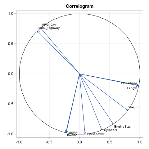
The correlogram is very similar to the loading plot from factor analysis. One difference is that the correlogram is rotated about 47 degrees as compared to the loadings plot. Because we only care about the angles between vectors (not the absolute angles), the rotation is not important. The other main difference is that the vectors in the correlogram are unit vectors whereas the vectors in the loadings plot are not. Otherwise, the facts that are apparent in the loadings plot are also apparent in the correlogram.

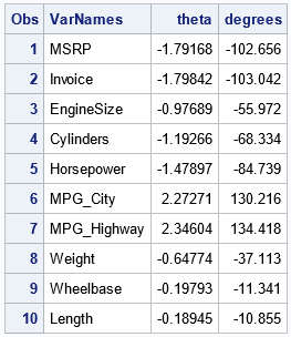
If you want to see the actual angles that were determined to be optimal, you can print the Correlogram data set:

proc print data=Correlogram;
   var varNames theta degrees;
run;

Summary

One way to visualize a matrix of correlations is to display a set of 2-D vectors such that the cosine of the pairwise angles between the vectors are approximately the same as the pairwise correlation (Trosset, 2005). This article uses PROC IML to implement a SAS macro that displays the correlogram for numerical variables in a SAS data set.

Further reading

Trosset, M. (2005), "Visualizing Correlation," Journal of Computational and Graphical Statistics