This article looks at a geometric method for estimating the center of a multivariate point cloud. The method is known as convex-hull peeling. In two-dimensions, you can perform convex-hull peeling in SAS 9 by using the CVEXHULL function in SAS IML software. For higher dimensions, you can use the CONVEXHULL subroutine, which was released in SAS IML as part of SAS Viya 2023.04.

Where is the center of multivariate data?

For univariate data, the mean and median statistics are commonly used to estimate the center of a distribution. The mean is easy to compute, but it is not robust to outliers. In contrast, the median is a robust statistic. It is easy to define the sample median for univariate data: you simply sort the data and then choose either the middle data value or the average of the two middle values.

For multivariate data, it is much harder to come up with a good robust statistic for the "middle" of the data. The mean and the geometric median are not robust. My favorite robust method is to the minimum covariance determinant (MCD) algorithm, which is available in SAS by using the MCD function in PROC IML or by using PROC ROBUSTREG in SAS/STAT software.

Prior to the development of the robust estimators, researchers proposed using geometric methods such as convex hulls to estimate the center of a multivariate data. Tukey (1975) introduced the concept of the depth of a point inside a point cloud. Then Barnett (1976, "The ordering of multivariate data") defined the convex hull ordering, which led to the idea of estimating the center of multivariate data by peeling the convex hull.

Peeling the convex hull

Peeling is an iterative algorithm. First, compute the convex hull. Then, remove the points on the boundary of the convex hull. You now have a smaller set of points. Iterate the process a certain number of times or until d+1 or fewer points remain, where d is the number of variables in the data. Lastly, take the average of the remaining points. That average is an estimate of the middle of the data.

Convex-hull peeling is a generalization of finding a median for univariate data. To see this, suppose we have eight sorted data values: 10, 12, 13, 13, 15, 20, 28, 57. By inspection, the median value is the average of the two middle values (13 and 15), but let's apply the convex-hull peeling algorithm to these one-dimensional data. The convex hull in one dimension is simply the union of the minimum and maximum data value.

1. First, find the convex hull of the original data, which is the set {10, 57}.
2. Next, remove the points on the convex hull. The new set is {12, 13, 13, 15, 20, 28}.
3. Repeat the process. The convex hull is {12, 28}. After removing these points, the remaining values are {13, 13, 15, 20}.
4. Repeat again. The convex hull is {13, 20}. After removing these points, the remaining values are {13, 15}.
5. At this point, only two points remain, which is the stopping criterion for d=1. The average of the remaining points is 14, which is the median.

Notice that the process associates to each observation the iteration at which it is removed. We call this the depth of the observation. Extreme values such as 10 and 57 have a small depth. Values that are near the center of the data (such as 13 and 15) have a large depth. If you think about it, the depth is like a quantile value, except that the depth is associate with both a low quantile (α) and a high quantile (1-α).

Convex-hull peeling in two dimensions

There are many applications in which estimating the middle of multivariate data is important. On application is in conservation biology. Suppose researchers are trying to map the habitat of a far-ranging animal such as a wolf. The center of the habitat might be a good place to search for the animal or its den. The following data represents hypothetical easting and northing coordinates (in km) for the wolf sightings. A call to PROC SGPLOT visualizes the locations:

data Wolf;
label x = "Easting (km)" y = "Northing (km)";
input x y @@;
datalines;
26   43.5  7   22    0   29    3   28.5 11   33.5 
17   22   17   36.5 11.5 29   21   39.5 27   35 
 8   34.5 11   31.5 19.5 35   20   39   24   53.5 
19   37   16.5 34.5 16.5 25.5 13.5 31.5 22.5 47 
17.5 38   15.5 36   28   46   20.5 37.5 37   48.5 
12.5 30    1   22.5 45.5 22   44.5 11.5 23   39 
31.5 26    7   24.5 41.5 13.5 57    9.5 14.5 21 
79   0 
;
 
title "Sightings of a Wolf";
proc sgplot data=Wolf;
   scatter x=x y=y;
   xaxis grid;
   yaxis grid;
run;

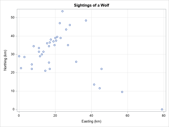
The graph shows that the about 30 sightings are along a northeast-by-southwest direction, but six sightings (possibly outliers?) are along a southeast direction. If you use PROC MEANS to compute the mean of the X and Y coordinates, you find that the mean is (21.8, 30.9). The mean value appears to be near the center of the point cloud, but perhaps the mean is unduly influenced by the possible outliers. Let's use convex-hull peeling to estimate the center of the data. If you are not familiar with the output of the CVEXHULL function, see the article, "Two-dimensional convex hulls in SAS."

The following SAS IML program defines a function called PEELCH, which implements the convex-hull peeling of a 2-D point cloud. The input and output arguments are:

• x is an n x 2 matrix, where each row is a point in 2-D.
• maxDepth is an integer that specifies the maximum number of times to iterate the convex-hull peeling. By default, maxDepth=50, but the algorithm might terminate in fewer iterations.
• The output of the function is an n x 2 matrix of polygons. The third column is an ID variable that identifies each polygon. The first and second columns are (x,y) pairs. The pairs are the same as for the x matrix, but for the i_th value of the ID variable, the (x,y) pairs are the vertices of the convex hull at depth i. The output is in the form expected by the POLYGON statement in PROC SGPLOT.

proc iml;
start peelCH(x, maxDepth=50);
   if ncol(x) ^= 2 then return(.);
   poly = j(nrow(x), 3, .);     /* return polygons: (px, py, ID) */
   currIdx = 1;                 /* keep track of current row */
   z = x;
   do i = 0 to maxDepth while(ncol(z) > 0);
      b = cvexhull(z);                     /* compute convex hull */
      idxBdry =  b[loc(b>0), ];            /* positive indices (always nonempty) */
      c = z[ idxBdry,];                    /* c = points on boundary of convex hull */
      lastIdx = currIdx + nrow(c) - 1;
      /* save polygon; use depth as the ID variable */
      poly[currIdx:lastIdx, ] = c || j(nrow(c), 1, i);   
      currIdx = lastIdx + 1;
      /* strip off outer hull; if points remain, continue iterating */
      idxInside = setdif(1:nrow(z), idxBdry);     /* interior indices */
      if ncol(idxInside) > 0 then 
         z = z[idxInside, ];               /* peel off outer convex hull */
      else                                 /* CH contains all remaining points */
         free z;
   end;
   return( poly );
finish;
 
/* call the peelCH function on the wolf data */
use Wolf;  read all var {x y} into x;  close;
poly = peelCH(x);
 
/* find the points at the maximum depth and average them */
maxDepth = max(poly[, 3]);
deepestPoints = poly[loc(poly[,3]=maxDepth), 1:2];
medianEst = mean( deepestPoints );
print medianEst;
 
/* write the convex hulls and the median estimate to data sets */
call symputx("maxDepth", maxDepth);         /* create macro variable of maximum depth */
create Hull from poly[c={'px' 'py' 'ID'}]; append from poly; close;
create Median from MedianEst[c={'mx' 'my'}]; append from MedianEst; close;
QUIT;

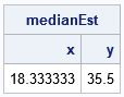
The peeling algorithm produces an estimate of (18.3, 35.5) for the median of these 2-D data. Recall that the mean of the coordinates is (21.8, 30.9), so the median is north and west of the mean by almost 6 km. This is because the median is less affected by the extreme observations in the southeast corner of the wolf's domain.

For the 2-D problem, you can use the POLYGON statement in PROC SGPLOT to visualize the peeling process:

data Peel;
   set Wolf Hull Median;
run;
 
title "Peeled Convex Hull";
title2 "Max depth = &maxDepth";
proc sgplot data=Peel noautolegend;
   polygon x=px y=py ID=ID / fill outline transparency=0.4;
   scatter x=x y=y;
   scatter x=mx y=my / markerattrs=(symbol=StarFilled size=12);
   xaxis grid;
   yaxis grid;
run;

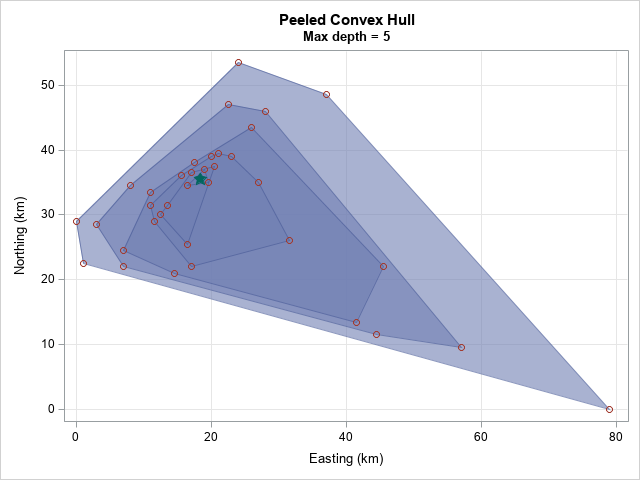
The image shows the initial convex hull of the data (depth=0) and the convex hulls after peeling away the first, second, third, and fourth layers. The deepest layer contains three points. The green star indicates the average of those three points. It is an estimate of the 2-D median for these data.

Convex hulls in higher dimensions

Convex hulls can be computed for higher-dimensional examples. The CONVEXHULL subroutine in SAS IML in SAS Viya can compute convex hulls for up to seven-dimensional data. That means that you can peel the convex hull for data sets that have up to seven numeric variables.

Summary

One early attempt to develop robust estimates of location for multivariate data was to iteratively peel the convex hull of multivariate data. Although this method is no longer in vogue, it remains an intriguing idea that is easy to understand and to visualize for 2-D data. This article demonstrates the convex-hull peeling algorithm for two-dimensional data. My previous article on the MCD algorithm provides a different way to obtain a robust statistical estimate of the center for multivariate data.