Given a set of N points in k-dimensional space, can you find the location that minimizes the sum of the distances to the points? The location that minimizes the distances is called the geometric median of the points. For univariate data, the "points" are merely a set of numbers $\{p_1, p_2, \ldots, p_N\}$, and it is well known that the sample median is the minimizer of the function $f(x) = \Sigma_i |p_i - x|$.

For two-dimensional data (points in the plane), you can find an exact solution for N=3 and N=4 points. For N=3, the geometric median of a triangle has an exact solution. For N=4, the convex hull of the points is generically a triangle or a quadrilateral, and the geometric median is known for both cases. For N > 4, there is no general direct method for computing the geometric median. Similarly, there is no direct method in higher dimensions.

There are, however, iterative methods that converge to the geometric median. This article shows how to compute the geometric median in SAS for an arbitrary set of points in arbitrary dimensions. One way is to use the conic optimization solver in PROC OPTMODEL. The conic optimization solver is available in SAS Viya. A second way is to use the SAS IML matrix language to implement the Ostresh (1978) modification of the Weiszfeld's (1937) iterative algorithm for computing the geometric median. Weiszfeld's algorithm is straightforward to implement in a matrix language.

The geometric median

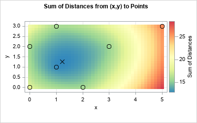
The geometric median is easiest to visualize for two-dimensional points in the plane. (If you haven't previously thought about the geometric median, you might want to start by thinking about the geometric median of a triangle.) The graph to the right shows the main idea for N = 7 points, represented by circles in the graph. For any point x = (x,y), let $f(\mathbf{x}) = \Sigma_i^N \| \mathbf{x} - \mathbf{p}_i \|$ be the sum of the Euclidean distances from x to the N points $\{\mathbf{p}_1, \mathbf{p}_2, \ldots, \mathbf{p}_N\}$. You can visualize the function by using a heat map, as shown in the graph. You can see that sum of the distances from (0,0) to the points is about 16 units (a green color), whereas the sum of the distances from (5,0) to the points is about 27 units (a red color). The sum of distances is minimized for points that are near the center of the cloud of points. The points colored in blue have the smallest distances. The location that has the minimum sum of distances is near (1.23, 1.26), which is indicated by an X. This point is the geometric median of the seven observations.

In some applications, we want to minimize a sum of costs rather than distances. In the simplest case, the cost is proportional to the distance, and the cost function can be represented as a weighted sum of distances.

The example generalizes in a natural way to higher-dimensional data. If you have N points in k-dimensional space, the geometric median is the point that minimizes the sum of the Euclidean distances to the N points.

Use the conic optimization solver to estimate the geometric median

If you use SAS Viya (LTS 2022.09), you can use the conic optimization solver in PROC OPTMODEL to approximate the geometric median by minimizing the sum of the distances. (LTS 2023.03 provides an additional enhancement: the automated conic transformation.) One of the examples in the documentation for PROC OPTMODEL shows the technique. I have slightly modified the example to find the geometric median for the seven points in the previous picture:

/* In SAS Viya LTS 2022.09, PROC OPTMODEL supports computing geometric medians 
   https://go.documentation.sas.com/doc/en/sasstudiocdc/v_037/pgmsascdc/casmopt/casmopt_conicsolver_examples02.htm
*/
%let n = 7;
%let k = 2;
proc optmodel;
   var x, y;                               * let (x, y) be the geometric median ;
   var d{1..&n} >= 0;                      * let d[i] = distance from geometric median to each sample point ;
   minimize f = sum{i in 1..&n}d[i];       * minimize the sum of distances ;
 
   * define the sample points ;
   num samples{1..&n, 1..&k} = [0 0, 2 0, 1 1, 1 3, 0 2, 3 2, 5 3 ];
   * calculate each distance ;
   con distance{i in 1..&n}: soc(d[i], (x-samples[i,1]) (y-samples[i,2]));
   expand;
 
   solve with conic;
   print x y;                              * print the optimal solution ;
quit;

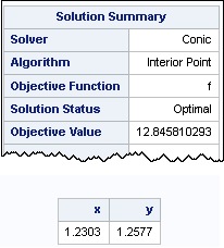
PROC OPTMODEL estimates the geometric median of the seven points at (1.23, 1.26). The objective function (sum of the distances) at that point is 12.8458. The solver formulates the problem by using a system of 9 variables that has 7 constraints. See the documentation for details.

Use Weiszfeld's algorithm to estimate the geometric median

An alternative way to find the geometric median is to use SAS IML to implement Weiszfeld's (1937) iterative algorithm for computing the geometric median. Weiszfeld's algorithm is a steepest gradient descent algorithm. If you write down the gradient of the objective function, you can construct an iterative method that converges to the minimum of the objective function. The details are in Ostresh's (1978) paper, which points out that Weiszfeld's algorithm should be modified to ensure that the iterative process never hits one of the data points.

The SAS IML program uses the following user-defined functions:

• IndexRowNoMatch: To avoid a technical problem in Weiszfeld's original algorithm, this function checks whether the estimate of the geometric median is one of the data points. It returns the indices to the data points that are different from the estimate.
• SumDist: The objective function. It returns the sum of the distance from an arbitrary point to the data points.
• UpdateGeoMedian: Implement one step in Weiszfeld's algorithm. Given a point, the function returns another point that is "downhill" from the input point in the direction of the gradient vector.
• GeoMedian: The main driver routine. The function uses the relative change of the objective function to determine convergence, but you could implement more sophisticated convergence criteria. It uses the centroid of the data points as an initial guess. It iterates the initial guess until convergence and returns the result.

/******** GEOMETRIC MEDIAN OF N-D POINTS ************************/
/* Implement the Ostresh (1978) variation of the Weiszfeld (1937) 
   algorithm for the geometric median of k-dimensional points.
   Ostresh, L. M. (1978) "On the Convergence of a Class of 
      Iterative Methods for Solving the Weber Location Problem"
      Operations Research, 26(4), pp. 597-609
      https://www.jstor.org/stable/169721
/****************************************************************/
 
proc iml;
/* for a matrix, X, return the rows of X that are not all zero */
start IndexRowNoMatch0(X);
   count = (X=0)[,+];          /* count number of 0s in each row */
   idx = loc(count<ncol(X));   /* at least one elements in row is not 0 */
   return idx;
finish;
/* For a matrix, X, return the rows of X that are not equal to a target vector.
   By default, the vector is the zero vector j(1, ncol(X), 0). */
start IndexRowNoMatch(X, target=);
   if IsSkipped(target) then 
      return IndexRowNoMatch0(X);
   else 
      return IndexRowNoMatch0(X-target);
finish;
 
/* Return the sum of weighted distances from m to rows of P.
   The rows of P are reference points. The point m is an 
   arbitrary point.
*/
start SumDist(m, P, wt=j(nrow(P),1,1));
   dist = distance(P, m);    /* dist from each row to m */
   return sum(wt # dist);    /* sum of the weighted distances */
finish;
 
/* Implement one step in Weiszfeld's iterative algorithm to 
   find the geometric median. This function assumes that 
   no row of P equals m. */
start UpdateGeoMedian(m, P, wt);
   dist = distance(P, m);    /* dist from each row to m */
   w = wt / dist;            /* scaled weights (avoid zeros in dist!) */
   mNew = w`*P / sum(w);     /* new estimate for geometric median */
   return mNew;
finish;
 
/* Implement Ostresh's modification of Weiszfeld's iterative algorithm to 
   find the geometric median. 
   Input:
      P: The rows of P specify the reference points.
      PrintIter: Specify PrintIter=1 to display the iteration history.
      wt: (optional) Specify a column vector of weights if you want a weighted median 
   Output: An estimate of the geometric median of the reference points
*/
start GeoMedian(P, PrintIter=0, wt=j(nrow(P),1,1));
   MaxIt = 100;     /* maximum number of iterations */
   FCrit = 1E-6;    /* criterion: stop when |fPrev - f| < FCrit */
   k = ncol(P);     /* dimension of points */
   n = nrow(P);     /* number of points points */
   m = (wt`*P)[:,] / sum(wt);  /* initial guess is weighted centroid */
 
   IterHist = j(MaxIt+1, k+1, .);
   IterHist[1,] = m || sum(distance(P,m));
   converged = 0;
   do i = 1 to MaxIt until(converged);
      mPrev = IterHist[i, 1:k];        /* previous guess for m */
      fPrev = IterHist[i, k+1];        /* previous sum of distances */
      idx = IndexRowNoMatch(P, m);     /* is the guess a data point? */
      if ncol(idx)=n then
         m = UpdateGeoMedian(m, P, wt);             /* no, use all points */
      else
         m = UpdateGeoMedian(m, P[idx,], wt[idx,]); /* yes, exclude the point */
      f = SumDist(m, P, wt);           /* evaluate the objective function */
      fDiff = abs(fPrev - f) / f;      /* relative change in function value */
      converged = (fDiff < FCrit);     /* has algorithm converged? */
      IterHist[i+1,] = m || f;         
   end;
   if PrintIter then do;
      IterHist = T(0:i) || IterHist[1:i+1,];
      colNames = 'Iter' || ('x1':strip('x'+char(k))) || 'Sum Dist';
      print IterHist[c=colNames L="Iteration History"];
   end;
   return m;
finish;
store module=(IndexRowNoMatch0 IndexRowNoMatch SumDist UpdateGeoMedian GeoMedian);
QUIT;

With these helper functions defined, you can call the GeoMedian function to find the geometric median of a set of points. The following program uses the same seven points as the previous sections:

proc iml;
load module=_all_;
 
/* N=7 points in 2-D */
P = {0 0, 2 0, 1 1, 1 3, 0 2, 3 2, 5 3};
gm = GeoMedian(P, 1);       /* estimate the geometric median and print iteration history */
sumDist = SumDist(gm, P);   /* get the sum of distances */
print gm[L='Geometric Median'],
      sumDist[L='Sum of Distances'];

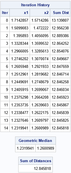
The output includes the iteration history for the algorithm. The initial guess is the geometric mean (centroid). For a nearly symmetric arrangement of points, the geometric mean and the geometric median should be close to each other. The algorithm improves the objective function at each step by moving in the negative gradient direction, which is the direction of steepest descent. By the fifth iteration, the objective function is changing slowly because it is somewhat flat near the minimum value. Over the remaining iterations, the algorithm slowly refines the point until the relative change of the function is less than 1E-6. The function returns (1.232, 1.260) as the estimate for the geometric median. The objective function at that point is 12.8458. This is very close to the solution obtained by using PROC OPTMODEL.

The weighted geometric median

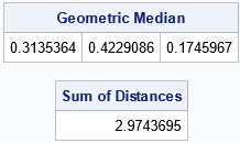
As mentioned earlier, some applications require minimizing a cost instead of the distance. When the cost can be expressed as a multiple of the distance, you obtain the weighted geometric median. For example, suppose the cost of moving goods from the points (1,3), (3,2), and (5,3) is proportional to twice the distance. Then you can assign these points a weight of 2 and assign the other points a weight of 1. Intuitively, you expect the weighted median to move closer to the points that have more weight. The following SAS IML statements compute the weighted geometric median:

/* perform a weighted computation */
wt = {1,1,1,2,1,2,2};
gmWt = GeoMedian(P, 0, wt);     /* estimate the weighted geometric median */
sumDist = SumDist(gmWt, P, wt); /* the weighted sum of distances */
print gmWt[L='Weighted Geo Median'],
      sumDist[L='Weighted Sum of Distances'];

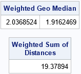
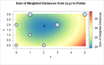
As expected, the geometric median is closer to the heavily weighted observations. You can create a graph that shows the objective function for the weighted geometric median. I have used a bubble plot to display the locations of the reference points. The size of each bubble is proportional to its weight.

The geometric median in higher dimensions

The SAS IML program can handle data in arbitrary dimensions. For example, the following program computes the geometric median of four points in three-dimensional space:

/* 3-D points */
P = {0.8 -0.2 0, 
     0.3  1   0,
     0    0   0,
     0.3  1   1};
gm = GeoMedian(P);          /* estimate the geometric median */
sumDist = SumDist(gm, P);   /* get the sum of distances */
print gm[L='Geometric Median'],
      sumDist[L='Sum of Distances'];

The performance of Weiszfeld's algorithm for the geometric median

The SAS IML computation for the geometric median is very fast. For example, the following DATA step creates 100,000 points in 10-dimensional space. The call to PROC IML reads the data and computes the geometric median.

/* create data set with k variables and N observations */
%let N = 100000;
%let k = 10;
data Sim;
array x[&k];
call streaminit(123);
do i = 1 to &N;
   do j = 1 to &k;
      x[j] = rand("Normal");
   end;
   output;
end;
drop i j;
run;
 
/* test the performance on large data */
proc iml;
load module=_all_;
 
use Sim; read all var _NUM_ into X; close;  /* read the data */
 
t0 = time();
gm = GeoMedian(X);        /* compute the geometric median */
time = time() - t0;
print time[F=5.3];

This computation of the geometric median completes for the 100,000 points in 0.03 seconds. The algorithm is linear in the number of observations, so it takes about 0.003 seconds for 10,000 observations and about 0.3 seconds for one million observations.

Summary

This article describes two ways to compute the geometric median of a set of reference points. The geometric median is the point that minimizes the sum of the distances to the reference points. One way to compute the geometric median is to use the conic optimization solver in PROC OPTMODEL in SAS Viya. A second way is to use the SAS IML matrix language to implement Ostresh's (1978) modification of Weiszfeld's (1937) iterative algorithm for computing the geometric median. Weiszfeld's algorithm uses iterations of matrix operations. If properly implemented, it can compute the geometric median for hundreds of thousands of points in a fraction of a second.

You can download the complete SAS program that I used to create the tables and graphs in this article.