On Twitter, I saw a tweet from @DataSciFact that read, "The sum of (x_i - x)^2 over a set of data points x_i is minimized when x is the sample mean." I (@RickWicklin) immediately tweeted out a reply: "And the sum of |x_i - x| is minimized by the sample median!"

It occurred to me that you can write a simple SAS program that demonstrates the @DataSciFact tweet and my response. This article creates graphs that show that the sample mean is the value that minimizes a quadratic loss function. Similarly, the sample median minimizes an absolute-difference loss function.

This demonstration can be surprising to students of statistics. In a beginning statistics course, the mean is presented in terms of a formula for an average. The median is defined as the midpoint of the set of ordered data values. It is not clear from these definitions that these estimates minimize some loss function.

Get the plotting range from the data

I am going to change notation from the original @DataSciFact tweet. Given univariate data {y1, y2, ..., yn}, the goal of this example is to plot two functions. The first function is the quadratic loss function
    Q(t) = Σ_i ( y[i]- t )²
The second function is similar but involves the sum of absolute values:
    A(t) = Σ_i | y[i]- t |
For both of these functions, the data values (y[i]) are fixed parameters, so these are univariate functions of t. The claim is that Q(t) reaches a minimum value when t equals the sample mean of the data, and A(t) is a minimum when t equals the sample median. The quadratic loss function is sometimes called the L2 loss function because it uses the L2 norm || y - t ||₂ for the data vector y. The other loss function is sometimes called the L1 loss function because it uses the L1 norm || y - t ||₁.

When you plot a function, you need to decide on the domain for the plot. Let's plot Q(t) on a domain that is centered at m, the mean of the data. A good choice is m ± s, where s is the standard deviation of the data. Similarly, you can plot A(t) on an interval that includes the median. One possible choice is the interquartile range [Q1, Q3], where Q1 is the first quartile (25th percentile) and Q3 is the third quartile (75th percentile).

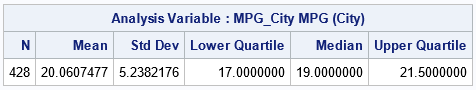
The following SAS statements call PROC MEANS to obtain the mean, standard deviation, and quartile of the data. I will use the MPG_City variable is the SasHelp.Cars data set, but you can modify the program to use any other data set and any other numerical variable. A subsequent DATA step creates macro variables that contain the statistics:

%let dsName = sashelp.cars;         /* specify any data set name */
%let varName = MPG_City;            /* specify any variable name */
 
/* Step 1: Get a suitable range for the variable */
proc means data=&dsName N Mean StdDev Q1 Median Q3;
   var &varName;
   output out=MeansOut mean=Mean stddev=StdDev q1=Q1 median=Median q3=Q3;
run;
 
/* create macro variables for mean, median, and range info */
data _null_;
set MeansOut;
call symputx('Mean', Mean);
call symputx('StdDev', StdDev);
call symputx('Q1', Q1);
call symputx('Median', Median);
call symputx('Q3', Q3);
run;

Plot the loss functions

This section plots the functions Q(t) and A(t) near the mean and median (respectively) of the data. To evaluate these functions by using the DATA step, you can transpose the data, which creates a data set that has one row and n columns that are named COL1, COL2, ..., COLn. You can then evaluate each function on an evenly spaced grid of values. The quadratic loss function is evaluated by summing the expression (y[i]- t)² over the data values for each value of t. Similarly, the absolute-difference loss function is evaluated by summing the expression | y[i]- t |.

/* PROC TRANSPOSE writes one row and columns COL1-COLn */
proc transpose data=&dsName out=Wide;   
   var &varName;
run;
 
data Results;
set Wide;
array y[*] COL:;             /* the data values */
 
/* L2 (quadratic) loss function */
Method = "L2";
do t = &Mean - &StdDev  to &Mean + &StdDev by 2*&StdDev/200;
   Loss = 0;
   do i = 1 to dim(y);
      Loss + (y[i] - t)**2;
   end;
   output;
end;
 
/* L1 (absolute value) loss function */
Method = "L1";
do t = &Q1 to &Q3 by (&Q3 - &Q1)/200;
   Loss = 0;
   do i = 1 to dim(y);
      Loss + abs(y[i] - t);
   end;
   output;
end;
keep Method t Loss;
run;

The data set contains the ordered pairs for each loss function. The following call to PROC SGPLOT graph the quadratic function on its domain:

title "Quadratic Loss Function";
proc sgplot data=Results(where=(Method='L2'));
   series x=t y=Loss;
   refline &Mean / axis=x label="Mean";
run;

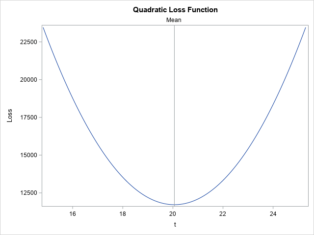
As promised, the quadratic loss function achieves a minimum value at t=20.06, which is the sample mean of the data. In this sense, the mean is a "least squares" minimizer. The graph shows that the sample mean is the value of t that minimizes the sum of the squared residuals between the data and t.

Next, let's graph the loss function for the absolute differences:

title "Absolute Loss Function";
proc sgplot data=Results(where=(Method='L1'));
   series x=t y=Loss;
   refline &Median / axis=x label="Median";
run;

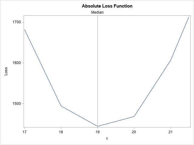
As promised, the absolute-difference loss function achieves a minimum value at t=19, which is the sample median of the data. In this sense, the median is the value of t that minimizes the sum of the magnitude of the residuals between the data and t. Notice that this graph is not smooth. It is piecewise linear between each data value.

Relationship with regression models

This article displays graphs that show how simple statistics (the sample mean and median) minimize certain "loss functions." You can generalize this idea to linear regression models. The regression coefficients for a least-squares model are estimated by values that minimize the sum of the squares of the residual values. The model predicts the (conditional) mean. The coefficients for a median-regression model (a type of quantile regression) are those that minimize the sum of the absolute values of the residual values. The model predicts the (conditional) median.

For a regression model that has two parameters (intercept and slope), the least-squares loss function is "bowl-shaped" and achieves a minimum for the least-squares estimates of the coefficients. The shape of the loss function for quantile regression is harder to visualize but shares many features of the one-dimensional example.

You can view the computations in this article as the result of running an intercept-only regression model. The least-squares estimate for an intercept-only model is the mean of the response variable. For a median regression model, the estimate for an intercept-only model is the median of the response variable. Consequently, you can get the mean and the median values by using the REG and QUANTREG regression procedures, respectively, to estimate an intercept-only model, as follows:

proc reg data=&dsName plots=none;
   model &varName = ;
   ods select ParameterEstimates;
quit;
 
proc quantreg data=&dsName;
   model &varName = / quantile=0.5; 
   ods select ParameterEstimates;
quit;

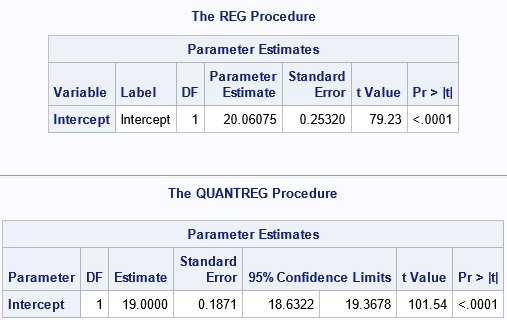
As anticipated, the estimate for the Intercept parameter from PROC REG is the mean. The estimate for the Intercept parameter from PROC QUANTREG is the median.

Summary

This article demonstrates a neat fact: The sum of (y[i]- t)² over a set of data points y[i]is minimized when t is the sample mean. Similarly, the sum of | y[i]- t | is minimized by the sample median!