In several previous articles, I've shown how to use SAS to fit models to data by using maximum likelihood estimation (MLE). However, I have not previously shown how to obtain standard errors for the estimates. This article combines two previous articles to show how to obtain MLE estimates and the standard errors for the estimates:

• "Two ways to compute maximum likelihood estimates in SAS" shows that you can use PROC NLMIXED to obtain MLE estimates, or you can "manually" solve the problem by using an optimization subroutine in PROC IML.
• "3 ways to obtain the Hessian at the MLE solution for a regression model" shows how to use SAS procedures to obtain a covariance matrix or, in some instances, the Hessian matrix of second derivatives for the log likelihood evaluated at the solution vector. The article discusses the relationship between these two matrices. If you are maximizing a log-likelihood function, the estimated covariance matrix for the parameters is the inverse of the negative Hessian matrix evaluated at the maximal solution. However, some SAS procedures minimize the NEGATIVE log likelihood. In that case, the covariance matrix is the inverse of the Hessian matrix.

Example: Fitting a lognormal distribution to data

As an example, let's reuse a previous example that fits parameters for a lognormal distribution to data. You can use PROC NLMIXED to obtain the MLE estimates. You can use the COV option to display the estimated covariance matrix for the parameters, as follows:

/* Create example Lognormal(2, 0.5) data of size N=200 */
%let N = 200;         
data LN;
call streaminit(98765);
zeta = 2;                  /* scale or log-location parameter */
sigma = 0.5;               /* shape or log-scale parameter    */
do i = 1 to &N;
   z = rand("Normal", zeta, sigma);  /* z ~ N(zeta, sigma)    */
   x = exp(z);                       /* x ~ LogN(zeta, sigma) */
   output;
end;
keep x;
run;
 
/* use MLE in PROC NLMIXED to fit a LN model to the data */
proc nlmixed data=LN COV;
   parms zeta 1 sigma 1;
   bounds 0 < sigma;
   LL = logpdf("Lognormal", x, zeta, sigma);
   model x ~ general(LL);
   ods select ParameterEstimates CovMatParmEst;
run;

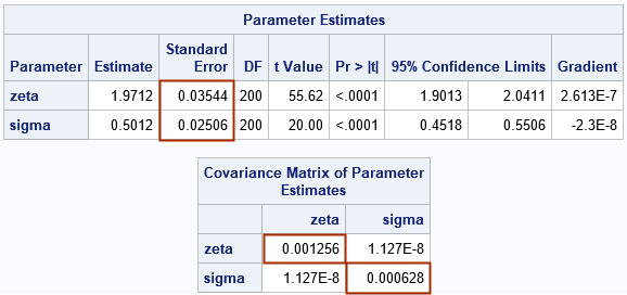
The output from PROC NLMIXED shows the MLE estimates and the standard errors (highlighted). As expected, the parameter estimates are close to the parameter values (2, 0.5) that are used to simulate the data. The output also shows the estimated covariance matrix of the parameters with the diagonal elements highlighted. You can verify that the standard error for each statistic is the square root of the corresponding variance element in the covariance matrix. For example, 0.03544 = sqrt(0.001256).

The NLMIXED procedure also supports the HESS option, which will display the Hessian matrix for the objective function at the optimal solution. The NLMIXED procedure minimizes the negative log likelihood. This means that the output of the HESS option will be the NEGATIVE of the Hessian that is displayed in the following section. The next section finds the maximal value for the (positive) log-likelihood (LL) function and computes the Hessian of the LL at that maximal value.

Explicitly solve the MLE problem

SAS procedures automatically take care of a lot of the underlying computational details so that you can focus on statistics and model-building. Nevertheless, it can be instructive to "manually" reproduce the output from a SAS procedure as a way of understanding the underlying mathematics of the problem. In this example, there is a log-likelihood function, which depends on the sample data. The MLE estimates are obtained by an optimization: find the parameter values that maximize the (log) likelihood that the data came from the specified distribution. In the SAS IML language, you can carry out these steps explicitly by defining the log-likelihood function and using an optimization routine (such as Newton-Raphson) to obtain the point that maximizes the log likelihood:

proc iml;
/* get the data, which are used for the LL computation */
use LN; read all var "x"; close;
 
/* log-likelihood function for lognormal data */
start LogNormal_LL(param) global(x);
   zeta  = param[1];
   sigma = param[2];
   LL = sum( logpdf("Lognormal", x, zeta, sigma) ); 
   return( LL );
finish;
 
/* create the constraint matrix */
con = { . 0,       /* lower bounds: 0 < sigma   */
        . .};      /* upper bounds:     N/A     */
opt = 1;           /* find maximum of LL function   */
param0  = {1 1};   /* initial guess for solution */
call nlpnra(rc, param_MLE, "LogNormal_LL", param0, opt, con); /* find optimal solution */
print param_MLE[c={"zeta" "sigma"}];

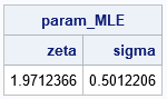
The output shows the parameter values that maximize the log-likelihood function. The output from PROC IML matches the parameter estimates from PROC NLMIXED.

If we want to get the standard errors for the parameter estimates, we can implement the following steps:

1. Compute the Hessian at the maximal MLE solution. You can use the NLPFDD subroutine in SAS 9.4 or the FDDSOLVE subroutine in SAS Viya to estimate the Hessian of the log-likelihood function at the optimal solution.
2. Compute the covariance matrix from the Hessian. If you are maximizing the log-likelihood function, then the covariance matrix is the inverse of the NEGATIVE Hessian: Cov = inv(-Hess). [Note: If you are minimizing the negative log-likelihood, then use Cov = inv(H_NLL), where H_NLL is the Hessian of the negative log-likelihood function, evaluated at the minimal point.]
3. Extract the diagonal elements (variances) from the covariance matrix and take the square root to obtain the standard errors.

These steps are implemented by using the following IML statements:

/* 1. Compute Hessian at the MLE solution. */
call nlpfdd(f, grad, Hess, "LogNormal_LL", param_MLE, {. 11}); /* '11' ==> central diff */
/* 2. Compute Cov matrix for parameters */
Cov = inv(-Hess);
/* 3. Extract diagonal elements (variances) and take square root */
stderr = sqrt(vecdiag(Cov));
 
parNames = {"zeta" "sigma"};
print Cov[r=parNames c=parNames], stderr[r=parNames];

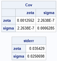
If you compare the covariance matrix and standard errors to the output from PROC NLMIXED, you will see that they are similar.

In general, you should see close agreement (a few decimal places) when you use PROC IML to solve the same MLE problem that a SAS procedure solves. It is unlikely that you will obtain exactly the same estimates (to full decimal precision) because the MLE estimate depends on the initial guess, the optimization algorithm, the convergence criterion, and other numerical factors. For the same reason, there will almost always be differences if you compare SAS results to the results from other statistical software.

Summary

This article shows how to obtain the standard errors for MLE parameter estimates. The example fits a two-parameter lognormal distribution to data, but the ideas apply to other MLE problems such as logistic regression, generalized linear regression models, and more. The main idea is to maximize the log-likelihood function to obtain the parameter estimates. You then evaluate the Hessian of the log-likelihood function at the optimal parameter values. You can estimate the covariance matrix of the parameters by taking the inverse of the NEGATIVE of the Hessian matrix. The standard errors are obtained by taking the square root of the diagonal elements of the covariance matrix.

You can also perform these computations by minimizing the negative of the log-likelihood function. In that case, the covariance matrix is the inverse of the Hessian evaluated at the minimal value.