3 ways to obtain the Hessian at the MLE solution for a regression model

When you use maximum likelihood estimation (MLE) to find the parameter estimates in a generalized linear regression model, the Hessian matrix at the optimal solution is very important. The Hessian matrix indicates the local shape of the log-likelihood surface near the optimal value. You can use the Hessian to estimate the covariance matrix of the parameters, which in turn is used to obtain estimates of the standard errors of the parameter estimates. Sometimes SAS programmers ask how they can obtain the Hessian matrix at the optimal solution. This article describes three ways:

For some SAS regression procedures, you can store the model and use the SHOW HESSIAN statement in PROC PLM to display the Hessian.
Some regression procedures support the COVB option ("covariance of the betas") on the MODEL statement. You can compute the Hessian as the inverse of that covariance matrix.
The NLMIXED procedure can solve general regression problems by using MLE. You can use the HESS option on the PROC NLMIXED statement to display the Hessian.

The next section discusses the relationship between the Hessian and the estimate of the covariance of the regression parameters. Briefly, they are inverses of each other. You can download the complete SAS program for this blog post.

Hessians, covariance matrices, and log-likelihood functions

The Hessian at the optimal MLE value is related to the covariance of the parameters. The literature that discusses this fact can be confusing because the objective function in MLE can be defined in two ways. You can maximize the log-likelihood function, or you can minimize the NEGATIVE log-likelihood.

In statistics, the inverse matrix is related to the covariance matrix of the parameters. A full-rank covariance matrix is always positive definite. If you maximize the log-likelihood, then the Hessian and its inverse are both negative definite. Therefore, statistical software often minimizes the negative log-likelihood function. Then the Hessian at the minimum is positive definite and so is its inverse, which is an estimate of the covariance matrix of the parameters. Unfortunately, not every reference uses this convention.

For details about the MLE process and how the Hessian at the solution relates to the covariance of the parameters, see the PROC GENMOD documentation. For a more theoretical treatment and some MLE examples, see the Iowa State course notes for Statistics 580.

Use PROC PLM to obtain the Hessian

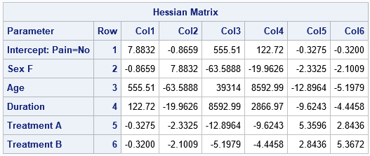
I previously discussed how to use the STORE statement to save a generalized linear model to an item store, and how to use PROC PLM to display information about the model. Some procedures, such as PROC LOGISTIC, save the Hessian in the item store. For these procedures, you can use the SHOW HESSIAN statement to display the Hessian. The following call to PROC PLM continues the PROC LOGISTIC example from the previous post. (Download the example.) The call displays the Hessian matrix at the optimal value of the log-likelihood. It also saves the "covariance of the betas" matrix in a SAS data set, which is used in the next section.

/* PROC PLM provides the Hessian matrix evaluated at the optimal MLE */
proc plm restore=PainModel;
   show Hessian CovB;
   ods output Cov=CovB;
run;

Not every SAS procedure stores the Hessian matrix when you use the STORE statement. If you request a statistic from PROC PLM that is not available, you will get a message such as the following: NOTE: The item store WORK.MYMODEL does not contain a Hessian matrix. The option in the SHOW statement is ignored.

Use the COVB option in a regression procedure

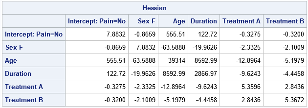
Many SAS regression procedures support the COVB option on the MODEL statement. As indicated in the previous section, you can use the SHOW COVB statement in PROC PLM to display the covariance matrix. A full-rank covariance matrix is positive definite, so the inverse matrix will also be positive definite. Therefore, the inverse matrix represents the Hessian at the minimum of the NEGATIVE log-likelihood function. The following SAS/IML program reads in the covariance matrix and uses the INV function to compute the Hessian matrix for the logistic regression model:

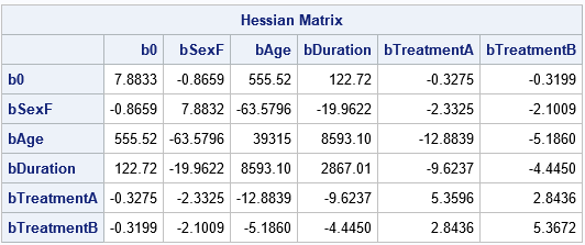
proc iml;
use CovB nobs p;                         /* open data; read number of obs (p) */
   cols = "Col1":("Col"+strip(char(p))); /* variable names are Col1 - Colp */
   read all var cols into Cov;           /* read COVB matrix */
   read all var "Parameter";             /* read names of parameters */
close;
 
Hessian = inv(Cov);                      /* Hessian and covariance matrices are inverses */
print Hessian[r=Parameter c=Cols F=BestD8.4];
quit;

You can see that the inverse of the COVB matrix is the same matrix that was displayed by using SHOW HESSIAN in PROC PLM. Be aware that the parameter estimates and the covariance matrix depend on the parameterization of the classification variables. The LOGISTIC procedure uses the EFFECT parameterization by default. However, if you instead use the REFERENCE parameterization, you will get different results. If you use a singular parameterization, such as the GLM parameterization, some rows and columns of the covariance matrix will contain missing values.

Define your own log-likelihood function

SAS provides procedures for solving common generalized linear regression models, but you might need to use MLE to solve a nonlinear regression model. You can use the NLMIXED procedure to define and solve general maximum likelihood problems. The PROC NLMIXED statement supports the HESS and COV options, which display the Hessian and covariance of the parameters, respectively.

To illustrate how you can get the covariance and Hessian matrices from PROC NLMIXED, let's define a logistic model and see if we get results that are similar to PROC LOGISTIC. We shouldn't expect to get exactly the same values unless we use exactly the same optimization method, convergence options, and initial guesses for the parameters. But if the model fits the data well, we expect that the NLMIXED solution will be close to the LOGISTIC solution.

The NLMIXED procedure does not support a CLASS statement, but you can use another SAS procedure to generate the design matrix for the desired parameterization. The following program uses the OUTDESIGN= option in PROC LOGISTIC to generate the design matrix. Because PROC NLMIXED requires a numerical response variable, a simple data step encodes the response variable into a binary numeric variable. The call to PROC NLMIXED then defines the logistic regression model in terms of a binary log-likelihood function:

/* output design matrix and EFFECT parameterization */
proc logistic data=Neuralgia outdesign=Design outdesignonly;
   class Pain Sex Treatment;
   model Pain(Event='Yes')= Sex Age Duration Treatment; /* use NOFIT option for design only */
run;
/* PROC NLMIXED required a numeric response */
data Design;
   set Design;
   PainY = (Pain='Yes');  
run;
 
ods exclude IterHistory;
proc nlmixed data=Design COV HESS;
   parms b0 -18 bSexF bAge bDuration bTreatmentA bTreatmentB 0;
   eta    = b0 + bSexF*SexF + bAge*Age + bDuration*Duration +
                 bTreatmentA*TreatmentA + bTreatmentB*TreatmentB;
   p = logistic(eta);       /* or 1-p to predict the other category */
   model PainY ~ binary(p);
run;

Success! The parameter estimates and the Hessian matrix are very close to those that are computed by PROC LOGISTIC. The covariance matrix of the parameters, which requires taking an inverse of the Hessian matrix, is also close, although there are small differences from the LOGISTIC output.

Summary

In summary, this article shows three ways to obtain the Hessian matrix at the optimum for an MLE estimate of a regression model. For some SAS procedures, you can store the model and use PROC PLM to obtain the Hessian. For procedures that support the COVB option, you can use PROC IML to invert the covariance matrix. Finally, if you can define the log-likelihood equation, you can use PROC NLMIXED to solve for the regression estimates and output the Hessian at the MLE solution.

Blogs