I recently gave a presentation about the SAS/IML matrix language in which I emphasized that a matrix language enables you to write complex analyses by using only a few lines of code. In the presentation, I used least squares regression as an example. One participant asked how many additional lines of code would be required for binary logistic regression. I think my answer surprised him. I claimed it would take about a dozen lines of code to obtain parameter estimates for logistic regression. This article shows how to obtain the parameter estimates for a logistic regression model "manually" by using maximum likelihood estimation.

Example data and logistic regression model

Of course, if you want to fit a logistic regression model in SAS, you should use PROC LOGISTIC or another specialized regression procedure. The LOGISTIC procedure not only gives parameter estimates but also produces related statistics and graphics. However, implementing a logistic regression model from scratch is a valuable exercise because it enables you to understand the underlying statistical and mathematical principles. It also enables you to understand how to generalize the basic model. For example, with minimal work, you can modify the program to support binomial data that represent events and trials.

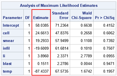
Let's start by running PROC LOGISTIC on data from the PROC LOGISTIC documentation. The response variable, REMISS, indicates whether there was cancer remission in each of 27 cancer patients. There are six variables that might be important in predicting remission. The following DATA step defines the data. The subsequent call to PROC LOGISTIC fits a binary logistic model to the data. The procedure produces a lot of output, but only the parameter estimates are shown:

data Remission;
   input remiss cell smear infil li blast temp;
   label remiss='Complete Remission';
   datalines;
1   .8   .83  .66  1.9  1.1     .996
1   .9   .36  .32  1.4   .74    .992
0   .8   .88  .7    .8   .176   .982
0  1     .87  .87   .7  1.053   .986
1   .9   .75  .68  1.3   .519   .98
0  1     .65  .65   .6   .519   .982
1   .95  .97  .92  1    1.23    .992
0   .95  .87  .83  1.9  1.354  1.02
0  1     .45  .45   .8   .322   .999
0   .95  .36  .34   .5  0      1.038
0   .85  .39  .33   .7   .279   .988
0   .7   .76  .53  1.2   .146   .982
0   .8   .46  .37   .4   .38   1.006
0   .2   .39  .08   .8   .114   .99
0  1     .9   .9   1.1  1.037   .99
1  1     .84  .84  1.9  2.064  1.02
0   .65  .42  .27   .5   .114  1.014
0  1     .75  .75  1    1.322  1.004
0   .5   .44  .22   .6   .114   .99
1  1     .63  .63  1.1  1.072   .986
0  1     .33  .33   .4   .176  1.01
0   .9   .93  .84   .6  1.591  1.02
1  1     .58  .58  1     .531  1.002
0   .95  .32  .3   1.6   .886   .988
1  1     .6   .6   1.7   .964   .99
1  1     .69  .69   .9   .398   .986
0  1     .73  .73   .7   .398   .986
;
 
proc logistic data=remission;
   model remiss(event='1') = cell smear infil li blast temp;
   ods select ParameterEstimates;
run;

The next section shows how to obtain the parameter estimates "manually" by performing a maximum-likelihood computation in the SAS/IML language.

Logistic regression from scratch

Suppose you want to write a program to obtain the parameter estimates for this model. Notice that the regressors in the model are all continuous variables, and the model contains only main effects, which makes forming the design matrix easy. To fit a logistic model to data, you need to perform the following steps:

1. Read the data into a matrix and construct the design matrix by appending a column of 1s to represent the Intercept variable.
2. Write the loglikelihood function. This function will a vector of parameters (b) as input and evaluate the loglikelihood for the binary logistic model, given the data. The Penn State course in applied regression analysis explains the model and how to derive the loglikelihood function. The function is
   $\ell(\beta) = \sum_{i=1}^{n}[y_{i}\log(\pi_{i})+(1-y_{i})\log(1-\pi_{i})]$
   where $\pi_i$ is the i_th component of the logistic transformation of the linear predictor: $\pi(\beta) = \frac{1}{1+\exp(-X\beta)}$
3. Make an initial guess for the parameters and use nonlinear optimization to find the maximum likelihood estimates. The SAS/IML language supports several optimization methods. I use the Newton-Raphson method, which is implemented by using the NLPNRA subroutine.

proc iml;
/* 1. read data and form design matrix */
varNames = {'cell' 'smear' 'infil' 'li' 'blast' 'temp'};
use remission;
read all var "remiss" into y;   /* read response variable */
read all var varNames into X;   /* read explanatory variables */
close;
X = j(nrow(X), 1, 1) || X;     /* design matrix: add Intercept column */
 
/* 2. define loglikelihood function for binary logistic model */
start BinLogisticLL(b) global(X, y);
   z = X*b`;                   /* X*b, where b is a column vector */
   p = Logistic(z);            /* 1 / (1+exp(-z)) */
   LL = sum( y#log(p) + (1-y)#log(1-p) );   
   return( LL );
finish;
 
/* 3. Make initial guess and find parameters that maximize the loglikelihood */
b0 = j(1, ncol(X), 0);         /* initial guess */
opt = 1;                       /* find maximum of function */
call nlpnra(rc, b, "BinLogisticLL", b0, opt);   /* use Newton's method to find b that maximizes the LL function */
print b[c=("Intercept"||varNames) L="Parameter Estimates" F=D8.];
QUIT;

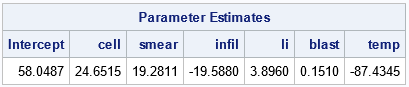
The parameter estimates from the MLE are similar to the estimates from PROC LOGISTIC. When performing nonlinear optimization, different software uses different methods and criteria for convergence, so you will rarely get the exact parameter estimates when you solve the same problem by using different methods. For these data, the relative difference in each parameter estimate is ~1E-4 or less.

I didn't try to minimize the number of lines in the program. As written, the number of executable lines is 16. If you shorten the program by combining lines (for example, p = Logistic(X*b`);), you can get the program down to 10 lines.

Of course, a program should never be judged solely by the number of lines it contains. I can convert any program to a "one-liner" by wrapping it in a macro! I prefer to ask whether the program mimics the mathematics underlying the analysis. Can the statements be understood by someone who is familiar with the underlying mathematics but might not be an expert programmer? Does the language provide analysts with the tools they need to perform and combine common operations in applied math and statistics? I find that the SAS/IML language succeeds in all these areas.

Logistic regression with events-trials syntax

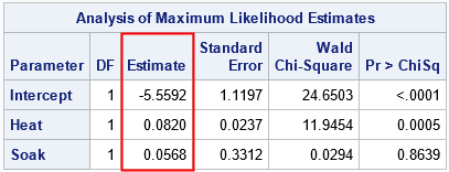
As mentioned previously, implementing the regression estimates "by hand" not only helps you to understand the problem better, but also to modify the basic program. For example, the syntax of PROC LOGISTIC enables you to analyze binomial data by using the events-trials syntax. When you have binomial data, each observation contains a variable (EVENTS) that indicates the number of successes and the total number of trials (TRIALS) for a specified value of the explanatory variables. The following DATA step defines data that are explained in the Getting Started documentation for PROC LOGISTIC. The data are for a designed experiment. For each combination of levels for the independent variables (HEAT and SOAK), each observation contains the number of items that were ready for further processing (R) out of the total number (N) of items that were tested. Thus, each observation represents N items for which R items are events (successes) and N-R are nonevents (failures).

The following DATA step defines the binomial data and calls PROC LOGISTIC to fit a logistic model:

/* Getting Started example for PROC LOGISTIC */
data ingots;
   input Heat Soak r n @@;
   datalines;
7 1.0 0 10  14 1.0 0 31  27 1.0 1 56  51 1.0 3 13
7 1.7 0 17  14 1.7 0 43  27 1.7 4 44  51 1.7 0  1
7 2.2 0  7  14 2.2 2 33  27 2.2 0 21  51 2.2 0  1
7 2.8 0 12  14 2.8 0 31  27 2.8 1 22  51 4.0 0  1
7 4.0 0  9  14 4.0 0 19  27 4.0 1 16
;
 
proc logistic data=ingots;
   model r/n = Heat Soak;
   ods select ParameterEstimates;
run;

Can you modify the previous SAS/IML program to accommodate binomial data? Yes! The key is "expand the data." Each observation represents N items for which R items are events (successes) and N-R are nonevents (failures). You could therefore reuse the previous program if you introduce a "frequency variable" (FREQ) that indicates the number of items that are represented by each observation.

The following program is a slight modification of the original program. The FREQ variable is derived from the EVENTS and TRIALS variables. The data is duplicated so that each observation in the binomial data becomes a pair of observations, one with frequency EVENTS and the other with frequency TRIALS-EVENTS. In the loglikelihood function, the frequency variable is incorporated into the summation.

proc iml;
/* 1. read data and form design matrix */
varNames = {'Heat' 'Soak'};
use ingots;
read all var "r" into Events;
read all var "n" into Trials;
read all var varNames into X;
close;
n = nrow(X);
X = j(n,1,1) || X;             /* design matrix: add Intercept column */
 
/* for event-trial syntax, split each data row into TWO observations,
   one for the events and one for the nonevents. Create Freq = frequency variable. */ 
Freq = Events // (Trials-Events);
X = X // X;                    /* duplicate regressors */
y = j(n,1,1) // j(n,1,0);      /* binary response: 1s and 0s */
 
/* 2. define loglikelihood function for events-trials logistic model */
start BinLogisticLLEvents(b) global(X, y, Freq);
   z = X*b`;                   /* X*b, where b is a column vector */
   p = Logistic(z);            /* 1 / (1+exp(-z)) */
   LL = sum( Freq#(y#log(p) + (1-y)#log(1-p)) );   /* count each observation numEvents times */
   return( LL );
finish;
 
/* 3. Make initial guess and find parameters that maximize the loglikelihood */
b0 = j(1, ncol(X), 0);         /* initial guess (row vector) */
opt = 1;                       /* find maximum of function */
call nlpnra(rc, b, "BinLogisticLLEvents", b0, opt);
print b[c=("Intercept"||varNames) L="Parameter Estimates" F=D8.];
QUIT;

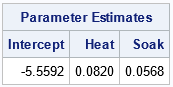
For these data and model, the parameter estimates are the same to four decimal places. Again, there are small relative differences in the estimates. But the point is that you can solve for the MLE parameter estimates for binomial data from first principles by using about 20 lines of SAS/IML code.

Summary

This article shows how to obtain parameter estimates for a binary regression model by writing about a short SAS/IML program. With slightly more effort, you can obtain parameter estimates for a binomial model in events-trials syntax. These examples demonstrate the power, flexibility, and compactness of the SAS/IML matrix programming language.

Of course, this power and flexibility come at a cost. When you use SAS/IML to solve a problem, you must understand the underlying mathematics of the problem. Second, the learning curve for SAS/IML is higher than for other SAS procedures. SAS procedures such as PROC LOGISTIC are designed so that you can focus on building a good predictive model without worrying about the details of numerical methods. Accordingly, SAS procedures can be used by analysts who want to focus solely on modeling. In contrast, the IML procedure is often used by sophisticated programmers who want to extend the capabilities of SAS by implementing custom algorithms.