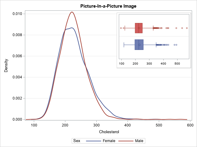
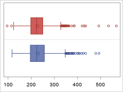
Did you know that you can embed one graph inside another by using PROC SGPLOT in SAS? A typical example is shown to the right. The large graph shows kernel density estimates for the distribution of the Cholesterol variable among male and female patients in a heart study. The small inset displays two box plots, which are an alternative visualization of the distributions.

There are three excellent papers that show how to display a small image inside a larger graph:

• Heath, Dan (2016), "Annotating the SAS ODS Graphics Way!" Dan shows how to use the SG annotation facility and the graph template language (GTL) to embed one graph inside another. He saves the smaller graph to a PNG file, then uses the Image function in the SG annotation facility to embed the PNG into a second graph. My article follow's Dan's ideas but uses PROC SGPLOT instead of the GTL.
• McConnell, Lelia (2016), "Picture-in-Picture - It’s Not Just for Television Anymore." Lelia shows how to use the LAYOUT OVERLAY and LAYOUTGRIDDED statements in GTL to overlay two graphs. On graph is large; the other is displayed in one cell of a 2 x 2 grid. If you are comfortable using GTL, this method is great because it does not require generating an image file.
• Kuhfeld, Warren (2017) "Advanced ODS Graphics: Inserting a graph into a graph." Warren shows three examples. The first uses PROC SGPLOT and the SG annotation facility. The other two examples discuss ODS graphs that are created by running statistical procedures in SAS/STAT software. My article follow's Warren's first example but uses a different method to save the small graph to a PNG file.

This article simplifies some of the methods in these papers and provides SAS code that you can use in SAS Studio and on remote servers when you do not have access to your local file system.

Steps to embed a graph

Following Heath (2016) and Kuhfeld (2017), this article uses the following steps to embed a small graph into a larger graph. The small graph is saved as a PNG image file. You can then use an SG annotation data set to embed the small image into the larger graph, as follows:

1. Decide where you will save the PNG image. Traditionally, this file is saved to your local file system, but if you are running SAS on a remote server or in the cloud, you might need to save the PNG to the WORK folder or some other libref for which you have write permission.
2. Generate the small graph and save it as a PNG file. If possible, use the ODS GRAPHICS / WIDTH= HEIGHT= options to create the graph at the size that you want it. Then the graph doesn't need to be resized when it is embedded. Rescaling can result in a blurry image.
3. Create an annotation data set that imports the image.
4. Create the large graph. Use the SGANNO= option on the PROC SGPLOT statement to read the annotation data set that embeds the small image.

Determine where to save an image file

You have two options for saving a PNG image file. You can save it to a local directory or to a temporary directory. Chris Hemedinger has shown how to create a temporary folder in the WORK libref or any other libref for which you have write permission. The two options are summarized below:

/* 1. Decide where you will save the PNG image. */
/* Option 1: Save graph to a local permanent location */
%let GPath = C:/Temp;
 
/* Option 2: save the PNG to a temporary directory. */
%let GPath = %sysfunc(getoption(WORK));  
 
/* In either case, ask SAS to create a subfolder: &GPath./images. See
   https://blogs.sas.com/content/sasdummy/2013/07/02/use-dlcreatedir-to-create-folders/ 
   You can skip this step if you are using a local folder.
*/
options dlcreatedir;
libname res "&GPath./images";    /* SAS will create this subfolder */
libname res clear;               /* done with libref, so clear it */

Save the small graph as an image file

The next step is to create a small graph and save it as a PNG file in the &GPath./images directory.

If you do an internet search for this topic, you are likely to find examples that use the ODS LISTING destination to create the small image. However, the LISTING destination might not use the same ODS style and attribute priorities as the destination that you are using. This can cause the small image to look different from what you expected.

An alternative is to use the same destination (and style) as you will use to create the large image. To do this, you can create a second ODS destination. When you create a second ODS destination, you can use the GPATH= option to specify the directory in which you want to put the image file.

You can use the ODS GRAPHICS option to set the size of the small graph. If possible, create the graph at the size you want it. (If necessary, you can rescale it when you embed it.) The following statements create a second ODS HTML destination and specify the GPATH= option. The PUSH option on the ODS GRAPHICS statement temporarily resets the width of the image to 240 pixels and specifies that it should be written to a PNG file named "MyGraph.png". After the graph is created, the POP option restores the ODS GRAPHICS environment. You can then close the second ODS destination.

/* 2. Generate the small graph and save it as a PNG file. 
   Generate it at the size that it needs to be. 
   You can open a second HTML dest by using ID=2: https://support.sas.com/kb/23/181.html
*/
ods html(2) gpath="&GPath./images" style=HTMLBlue;  /* specify a STYLE= option, if necessary */
* temporarily change the state of ODS graphics;
ods graphics / push reset width=240px imagefmt=PNG imagename="MyGraph";
* now create any graph and save the PNG to the directory;
title "Distribution by Sex";
proc sgplot data=Sashelp.Heart noautolegend;
   hbox Cholesterol / group=Sex;
   yaxis grid;
   xaxis display=(nolabel);
run;
* restore the state of ODS graphics and close destination;
ods graphics / pop;  
ods html(2) close;

Notice a few tricks here. I use the HTML destination, not the LISTING destination. I use the PUSH and POP options so that I do not corrupt my current ODS GRAPHICS environment. I create and close a secondary ODS destination so that I do not have to open/close my primary destination, which might interfere with my current working environment.

I do not completely understand why, but I want to point out that the PNG file might be named MyGraph1.png instead of MyGraph.png. When I run the previous code in SAS Studio in SAS Viya, the graph is named MyGraph.png. However, when I run the code in my PC in the SAS 9.4 windowing environment, the name is MyGraph1.png.

Use annotation to embed an image

As I explained in an earlier post, you can use the SG annotation macros to create an annotation data set that embeds an image in a graph. In this case, the image is the small graph that we created in the previous section. The name might be MyGraph.png (SAS Viya in SAS Studio) or MyGraph1.png (SAS 9.4 windowing environment).

/* 3. Create an annotation data set that imports the image. See
      https://blogs.sas.com/content/iml/2023/09/13/sg-annotation-macros.html
*/
%SGANNO;    /* compile the annotation macros (Do this only once.) */
data anno;
/* The name of the graph depends on your environment. 
   In SAS Studio, the graph is named MyGraph.png.
   On a PC in the SAS windowing environment, the name is MyGraph1.png. */
%SGIMAGE(image="&GPath./images/MyGraph1.png",    /* or "MyGraph.png" */
         drawspace="wallpercent", x1=55, y1=98,
         anchor="topleft",
         border="true"         
         /* if necessary, you can scale the image here:
         ,width=200,
         widthunit="pixel"  */
         );
run;
 
/* 4. Create the large image. Use the SGANNO= option to embed the smaller image. */
title "Picture-In-a-Picture Image";
proc sgplot data=Sashelp.Heart sganno=anno;
  density Cholesterol / type=kernel group=Sex;
  yaxis grid;
run;

The image is shown at the top of this article. The small graph is embedded in the upper left corner of the larger graph. You will probably need to try several values of the X1= and Y1= parameters in the %SGIMAGE macro before you find the right combination. The image is anchored at the point (X1,Y1) relative to a scale in which the "wall area" of the large graph is assigned the coordinate system [0,100] x [0,100]. Heath (2016, p. 2) shows the coordinate systems that you can use for SG annotation.

If you are writing the mage to a local directory, you might want to delete the PNG file after creating the larger graph. This optional step is left as an exercise.

Summary

This article shows how to embed one graph inside another by using PROC SGPLOT in SAS. You first decide where to save a PNG image, then generate a small graph as a PNG file. You then use an annotation data set to import the image into a larger graph. The method in this article works even if you are running SAS on a remote server or in the cloud.