The area of a convex hull enables you to estimate the area of a compact region from a set of discrete observations. For example, a biologist might have multiple sightings of a wolf pack and want to use the convex hull to estimate the area of the wolves' territory. A forestry expert might use a convex hull to estimate the area of a forest that has been infested by a beetle or a blight. This article shows how to compute the area and perimeters of convex hulls in SAS. Because a convex hull is a convex polygon, we present formulas for the area and perimeter of polygons and apply those formulas to convex hulls.
Gauss' shoelace formula for the area of a polygon
There are many formulas for the area of a planar polygon, but the one used in this article is known as
Gauss' shoelace formula, or the triangle formula.
This formula enables you to compute the area of a polygon by traversing the vertices of the polygon in order. The formula uses only the coordinates of adjacent pairs of vertices. Assume a polygon has n that are vertices enumerated counterclockwise, and the coordinates are
\((x_1, y_1), (x_2, y_2), \ldots, (x_n, y_n)\).
Then the area of the polygon is given by the shoelace formula
\(A = \frac{1}{2} \sum_{i=1}^{n} x_i y_{i+1} - x_{i+1} y_i\)
where we use the convention that \((x_{n+1}, y_{n+1}) = (x_1, y_1)\).
To me, the remarkable thing about this formula is that it looks like it has nothing to do with an area. However, the Appendix derives Gauss' shoelace formula from Green's theorem in the plane, which reveals the connection between the formula and the area of the polygon.
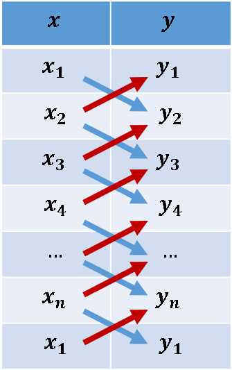
You might wonder why this is called the "shoelace formula." Suppose a polygon has vertices \((x_1, y_1), (x_2, y_2), \ldots, (x_n, y_n)\). A schematic visualization of the formula is shown to the right. You list the X and Y coordinates of the vertices and append the first vertex to the end of the list. The blue arrows represent multiplication. The red arrows represent multiplication with a negative sign. So, the first two rows indicate the quantity \(x_1 y_2 - x_2 y_1\). (If you are familiar with linear algebra, you can recognize this quantity as the determinant of the 2 x 2 matrix with first row \((x_1, y_1)\) and second row \((x_2, y_2)\).) The sequence of arrows looks like criss-cross lacing on a shoe.
Implementing the area and perimeter of a polygon in SAS
The visualization of the shoelace formula suggests an efficient method for computing the area of a polygon. First, append the first vertex to the end of the list of vertices. Then, define the vector Lx = lag(x) as the vector with elements \(x_2, x_3, \ldots, x_n, x_1\). Define Ly = lag(y) similarly. Then form the vector d = x#Ly – y#Lx, where the '#' operator indicates elementwise multiplication. The area of the polygon is the sum(d)/2. This computation is implemented in the following SAS/IML program, which also implements a function that computes the Euclidean distance along the edges of the polygon. The perimeter formula is given by\(s = \sum_{i=1}^{n} \sqrt{(x_{i+1} -x_i)^2 + (y_{i+1} -y_i)^2}\), where \((x_{n+1}, y_{n+1}) = (x_1, y_1)\).
proc iml; /* The following functions are modified from Rick Wicklin (2016). The Polygon package. SAS Global Forum 2016 */ /* PolyArea: Return the area of a simple polygon. P is an N x 2 matrix of (x,y) values for vertices. N > 2. This function uses Gauss' "shoelace formula," which is also known as the "triangle formula." See https://en.wikipedia.org/wiki/Shoelace_formula */ start PolyArea(P); lagIdx = 2:nrow(P) || 1; /* vertices of the lag; appends first vertex to the end of P */ xi = P[ ,1]; yi = P[ ,2]; xip1 = xi[lagIdx]; yip1 = yi[lagIdx]; area = 0.5 * sum(xi#yip1 - xip1#yi); return( area ); finish; /* PolyPerimeter: Return the perimeter of a polygon. P is an N x 2 matrix of (x,y) values for vertices. N > 2. */ start PolyPeri(_P); P = _P // _P[1,]; /* append first vertex */ /* (x_{i+1} - x_i)##2 + (y_{i+1} - y_i)##2 */ v = dif(P[,1])##2 + dif(P[,2])##2; /* squared distance from i_th to (i+1)st vertex */ peri = sum(sqrt(v)); /* sum of edge lengths */ return( peri ); finish; /* demonstrate by using a 3:4:5 right triangle */ Pts = {1 1, 4 1, 4 5}; Area = PolyArea(Pts); Peri = PolyPeri(Pts); print Area Peri; |

The output shows the area and perimeter for a 3:4:5 right triangle with vertices (1,1), (4,1), and (4,5). As expected, the area is 0.5*base*height = 0.5*3*4 = 6. The perimeter is the sum of the edge lengths: 3+4+5 = 12.
Notice that neither of the functions uses a loop over the vertices of the polygon. Instead, the area is computed by using vectorized computations. Essentially, the area formula uses the LAG of the vertex coordinates, and the perimeter formula uses the DIF of the coordinates.
Apply the area and perimeter formulas to convex hulls
You can use the previous functions to compute the area and perimeter of the 2-D convex hull of a set of planar points. In SAS, you can use the CVEXHULL function to compute a convex hull. The CVEXHULL function returns the indices of the points on the convex hull in counterclockwise order. You can therefore extract those points to obtain the polygon that encloses the points. You can send this polygon to the functions in the previous section to obtain the area and perimeter of the convex hull, as follows:
/* Use the CVEXHULL function in SAS to compute 2-D convex hulls. See https://blogs.sas.com/content/iml/2021/11/15/2d-convex-hull-sas.html */ points = {0 2, 0.5 2, 1 2, 0.5 1, 0 0, 0.5 0, 1 0, 2 -1, 2 0, 2 1, 3 0, 4 1, 4 0, 4 -1, 5 2, 5 1, 5 0, 6 0 }; /* Find the convex hull: indices on the convex hull are positive */ Indices = cvexhull( points ); hullIdx = indices[loc(indices>0)]; /* extract vertices with positive indices */ convexPoly = points[hullIdx, ]; /* extract rows to form a polygon */ print hullIdx convexPoly[c={'cx' 'cy'} L=""]; /* what is the area of the convex hull? */ AreaCH = PolyArea(convexPoly); PeriCH = PolyPeri(convexPoly); print AreaCH PeriCH; |
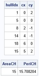
The output shows the indices and coordinates of the convex polygon that bounds the set of points. It is a two-column matrix, where each row represents the coordinates of a vertex of the polygon. The area of this polygon is 15 square units. The perimeter is 15.71 units. If these coordinates are the locations of spatial observations, you can compute the area and perimeter of the convex hull that contains the points.
Summary
A convex hull is a polygon. Accordingly, you can use formulas for the area and perimeter of a polygon to obtain the area and perimeter of a convex hull. This article shows how to efficiently compute the area and perimeter of the convex hull of a set of planar points.
Appendix: Derive Gauss' shoelace formula from Green's theorem
If a polygon has n vertices with coordinates \((x_1, y_1), (x_2, y_2), \ldots, (x_n, y_n)\), we
want to prove Gauss' shoelace formula:
\(A = \frac{1}{2} \sum_{i=1}^{n} x_i y_{i+1} - x_{i+1} y_i\)
where we use the convention that \((x_{n+1}, y_{n+1}) = (x_1, y_1)\).
At first glance, Gauss' shoelace formula does not appear to be related to areas. However, the formula is connected to area because of a result from multivariable calculus known as "the area corollary of Green's theorem in the plane." Green's theorem enables you to compute the area of a planar region by computing a line integral around the boundary of the region. That is what is happening in Gauss' shoelace formula. The "area corollary" says that you can compute the area of the polygon by computing \(\oint_C x/2\; dx - y/2\; dy\), where C is the piecewise linear path along the perimeter of the polygon.
Let's evaluate the integral on the edge between the i_th and (i+1)st vertex. Parameterize the i_th edge as
\((x(t), y(t)) = ( x_i + (x_{i+1}-x_i)t, y_i + (y_{i+1}-y_i)t )\quad \mathrm{for} \quad t \in [0,1]\).
With this parameterization,
\(dx = (dx/dt)\; dt = (x_{i+1}-x_i)\; dt\) and \(dy = (dy/dt)\; dt = (y_{i+1}-y_i)\; dt\).
When you substitute these expressions into the line integral, the integrand becomes a linear polynomial in t, but a little algebra shows that the linear terms cancel and only the constant terms remain. Therefore, the line integral on the i_th edge becomes
\(\frac{1}{2} \int_{\mathrm edge} x\; dx - y\; dy = \frac{1}{2} \int_0^1 x_i (y_{i+1}-y_i) - y_i (x_{i+1}-x_i) dt = \frac{1}{2} (x_i y_{i+1}- y_i x_{i+1})\).
When you evaluate the integral on all edges of the polygon, you get a summation, which proves Gauss' shoelace formula for the area of a polygon.
