Recently, I wrote about Bartlett's test for sphericity. The purpose of this hypothesis test is to determine whether the variables in the data are uncorrelated. It works by testing whether the sample correlation matrix is close to the identity matrix.

Often statistics textbooks or articles include a statement such as "under the null hypothesis, the test statistic is distributed as a chi-square statistic with DF degrees of freedom." That sentence contains a lot of information! Using algebraic formulas and probability theory to describe a sampling distribution can be very complicated. But it is straightforward to describe a sampling distribution by using simulation and statistical graphics.

This article discusses how to use simulation to understand the sampling distribution of a statistic under a null hypothesis. You can find many univariate examples of simulating a sampling distribution for univariate data, but this article shows the sampling distribution of a statistic for a hypothesis test on multivariate data. The hypothesis test in this article is Bartlett's sphericity test, but the ideas apply to other statistics. It also shows a useful trick for simulating correlation matrices for multivariate normal (MVN) data.

The simulation approach to null distributions

Simulation is well-suited for explaining the sampling distribution of a statistic under the null hypothesis. For Bartlett's sphericity test, the null hypothesis is that the data are a random sample of size N from a multivariate normal population of p uncorrelated variables. Equivalently, the correlation matrix for the population is the p x p identity matrix. Under this hypothesis, the test statistic
$T = -\log(\det(R)) (N-1-(2p+5)/6)$
has a chi-square distribution with p(p–1)/2 degrees of freedom, where R is the sample correlation matrix. In other words, if we randomly sample many times from an uncorrelated MVN distribution, the statistics for each sample will follow a chi-square distribution. Let's use simulation to visualize the null distribution for Bartlett's test.

Here is a useful fact: You do not have to generate MVN data if the statistic is related to the covariance or correlation of the data. Instead, you can DIRECTLY simulate a correlation matrix for MVN data by using the Wishart distribution. The following SAS/IML statements use the Wishart distribution to simulate 10,000 correlation matrices for MVN(0, Σ) samples, where Σ is a diagonal covariance matrix:

proc iml;
call randseed(12345);
p = 3;                               /* number of MVN variables */
N = 50;                              /* MVN sample size   */
Sigma = diag(1:p);                   /* population covariance */
NumSamples = 10000;                  /* number of samples in simulation */
 
/* Simulate correlation matrices for MVN data by using the Wishart distribution.
/* Each row of A is a scatter matrix; each row of B is a covariance matrix */
A = RandWishart(NumSamples, N-1, Sigma); /* N-1 degrees of freedom */
B = A / (N-1);                           /* rescale to form covariance matrix */
 
/* print one row to show an example */
C = shape(B[1,], p);                     /* reshape 1st row to p x p matrix */
R = cov2corr(C);                         /* convert covariance to correlation */
print C, R;

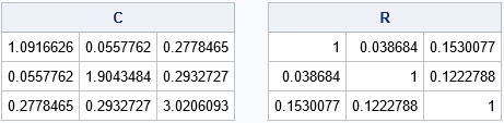
The output shows one random covariance matrix (C) and its associate correlation matrix (R) from among the 1,000 random matrices. The B matrix is 10000 x 9, and each row is a sample covariance matrix for a MVN(0, Σ) sample that has N=50 observations.

Recall that the determinant of a correlation matrix is always in [0,1]. The determinant equals 1 only when R=I(p). Therefore, the expression -log(det(R)) is close to 0 when R is close to the identity matrix and gets more and more positive as R is farther and farther away from the identity matrix. (It is undefined if R is singular.) So if we apply Bartlett's formula to each of the random matrices, we expect to get a lot of statistics that are close to 0 (because R should be close to the identity) and a few that are far away. The following SAS IML program carries out this method and plots the 10,000 statistics that result:

T = j(numSamples, 1);
do i = 1 to NumSamples;
   cov = shape(B[i,], p, p);             /* convert each row to square covariance matrix */
   R = cov2corr(cov);                    /* convert covariance to correlation */
   T[i] = -log(det(R)) * (N-1-(2*p+5)/6);
end;
 
title "Bartlett's Sphericity Statistic";
title2 "&numSamples MVN(0, Sigma) Samples for Diagonal Covariance";
call histogram(T) rebin={0.25 0.5};

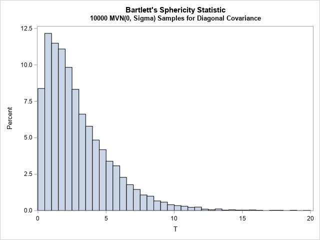
The histogram shows the null distribution, which is the distribution of Bartlett's statistic under the null hypothesis. As expected, most statistics are close to 0. Only a few are far from 0, where "far" is a relative term that depends on the dimension of the data (p).

Knowing that the null distribution is a chi-square distribution with DF=p(p-1)/2 degrees of freedom helps to provide a quantitative value to "far from 0." You can use the 95th percentile of the chi-square(DF) distribution to decide whether a sample correlation matrix is "far from 0":

/* critical value of chi-square(3) */
DF = p*(p-1)/2;
crit = quantile("ChiSq", 0.95, DF);  /* one-sided: Pr(chiSq < crit)=0.95 */
print crit;

You can overlay the chi-square(3) distribution on the null distribution and add the critical value to obtain the following figure:

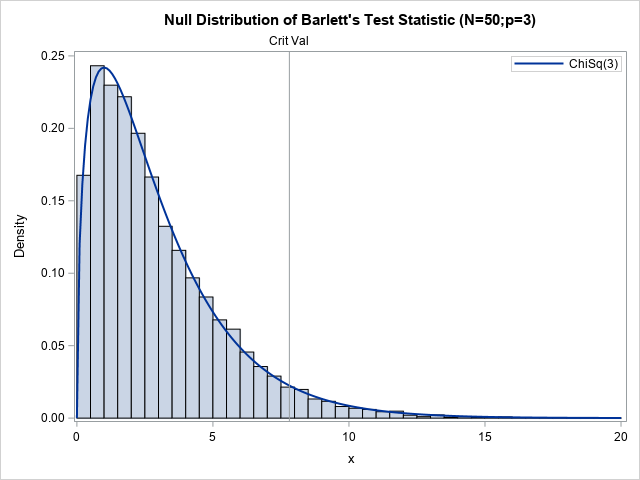
This graph summarizes the Bartlett sphericity test. The histogram approximates the null distribution by computing Bartlett's statistic on 10,000 random samples from an uncorrelated trivariate normal distribution. The curve is the asymptotic chi-square(DF=3) distribution. The vertical line is the critical value for testing the hypothesis at the 95% confidence level. The next section uses this graph and Bartlett's test to determine whether real data is a sample from an uncorrelated MVN distribution.

Bartlett's test on real data

The previous graph shows the null distribution. If you run the test on a sample that contains three variables and 50 observations, you will get a value of the test statistic. If the value is greater than 7.8, it is unlikely that the data are from an uncorrelated multivariate normal distribution.

A previous article showed how to use PROC FACTOR to run Bartlett's test in SAS. Let's run PROC FACTOR on 50 observations and three variables of Fisher's Iris data:

proc factor data=sashelp.iris(obs=50) method=ML heywood;
   var SepalLength SepalWidth PetalLength ;
   ods select SignifTests; /* output only Bartlett's test */
run;

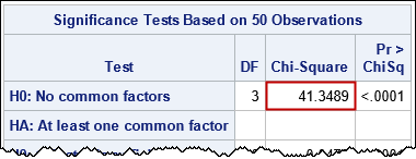
The value of Bartlett's statistic on these data is 41.35. The X axis for the null distribution only goes up to 20, so this value is literally "off the chart"! You would reject the null hypothesis for these data and conclude that these data do not come from the null distribution.

When researchers see this result, they often assume that one or more variables in the data are correlated. However, it could also be the case that the data are not multivariate normal since normality is an assumption that was used to generate the null distribution.

Summary

This article shows how to simulate the null distribution for Bartlett's sphericity test. The null distribution is obtained by simulating many data samples from an uncorrelated multivariate normal distribution and graphing the distribution of the test statistics. For Bartlett's test, you get a chi-square distribution.

The ideas in this article apply more generally to other hypothesis tests. An important use of simulation is to approximate the null distribution for tests when an exact form of the distribution is not known.

This article also shows that you can use the Wishart distribution to avoid having to simulate MVN data. If the goal of the simulation is to obtain a covariance or correlation matrix for MVN data, you can use the Wishart distribution to simulate the matrix directly.