When you have many correlated variables, principal component analysis (PCA) is a classical technique to reduce the dimensionality of the problem. The PCA finds a smaller dimensional linear subspace that explains most of the variability in the data. There are many statistical tools that help you decide how many principal components to keep.

However, not all data can benefit from a PCA. If the variables are weakly correlated, it might not be possible to reduce the dimension of the problem. Bartlett's sphericity test provides information about whether the correlations in the data are strong enough to use a dimension-reduction technique such as principal components or common factor analysis.

This article discusses Bartlett's sphericity test (Bartlett, 1951) and shows how to run it in SAS. I provide two examples: one uses strongly correlated data for which a PCA would be an appropriate analysis; the other uses simulated data for which the variables are uncorrelated. For the second example, Bartlett's test tells us that a dimension-reduction technique will not provide any useful benefit. You need all dimensions to explain the variance in the data.

Choose the correct "Bartlett test"

Be aware that there are two tests that have Bartlett's name, and they are similar. The better-known test is Bartlett's test for equal variance, which is part of an ANOVA analysis. It tests the hypothesis that the variances across several groups are equal. The technical term is "homogeneity of variance," or HOV. The GLM procedure in SAS can perform Bartlett's test for homogeneity of variance. The documentation has a discussion and example that shows how to use Bartlett's HOV test.

Bartlett's sphericity test is different. Loosely speaking, the test asks whether a correlation matrix is the identity matrix. If so, the variables are uncorrelated, and you cannot perform a PCA to reduce the dimensionality of the data. More formally, Bartlett's sphericity test is a test of whether the data are a random sample from a multivariate normal population MVN(μ, Σ) where the covariance matrix Σ is a diagonal matrix. Equivalently, the variables in the population are MVN and uncorrelated.

Bartlett's sphericity test for correlated data

Let's recall some facts about correlation matrices that are necessary to understand Bartlett's sphericity test. Assume the data matrix, X, has p variables and N > p observations. First, the determinant of a correlation matrix is always in the range [0,1]. The determinant equals 1 only when the correlation matrix is the identity matrix, which happens only if the columns The determinant equals 0 only when data are linearly dependent, which means that a column is equal to a linear combination of the other columns. Thus, for nondegenerate data, the determinant is always in the range (0,1] and the logarithm of the determinant is defined. Bartlett's sphericity statistic is
$T = -\log(\det(R)) (N-1-(2p+5)/6)$
Under the null hypothesis that the data are a random sample from the MVN(μ, Σ) distribution where the covariance matrix Σ is a diagonal matrix, Bartlett (1951) showed that this statistic has a chi-square distribution with p(p–1)/2 degrees of freedom.

If you look up "how to obtain Bartlett's test of sphericity in SAS," you will be directed to a SAS Usage note that consists of five brief sentences and a partial example. Here is a more complete example. Suppose you want to know whether a set of variables are correlated strongly enough that you can use a dimension-reduction technique to analyze the data. You can use PROC FACTOR in SAS to produce Bartlett's test. You need to specify the METHOD=ML (maximum likelihood estimation) and HEYWOOD options. The following example uses the Sashelp.Iris data, which contains four highly correlated variables. For these data, three correlation coefficients are greater than 0.8. The following statements produce Bartlett's sphericity test:

proc factor data=sashelp.iris method=ML heywood;
   ods select SignifTests; /* output only Bartlett's test */
run;

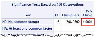
Bartlett's test is shown on the row labeled "H0: No common factors." These data have p=4 variables, so there are DF=6 degrees of freedom for the test. The value of the test statistic is 706.96. Under the null hypothesis, the probability of observing a statistic this large or larger by chance alone is exceedingly small. Therefore, you reject the null hypothesis and conclude that it is reasonable to consider applying a dimension-reduction technique to these data.

Bartlett's sphericity test for uncorrelated data

What does Bartlett's sphericity test look like if your sample is from an uncorrelated MVN distribution? Let's simulate three-dimensional uncorrelated MVN data and run the test:

data UncorrMVN;
call streaminit(123);
do i = 1 to 50;
   x1 = rand("Normal", 0, 1);
   x2 = rand("Normal", 0, 2);
   x3 = rand("Normal", 0, 3);
   output;
end;
drop i;
run;
 
proc factor data=UncorrMVN method=ML heywood;
   ods select SignifTests;
run;

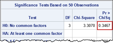
For these data (which are simulated according to the null hypothesis), the p-value is not small, so there is not enough evidence to reject the null hypothesis that the variables in the population are uncorrelated. For these data, you need three dimensions to fully capture the variance in the data. Therefore, a dimension-reduction technique is not a useful way to analyze these data.

Summary

You can run Bartlett's sphericity test in SAS by using PROC FACTOR and the METHOD=ML HEYWOOD options. The test is shown in the SignifTests ODS table. The null hypothesis is that the data are a sample from an uncorrelated MVN distribution. If the p-value of the test is less than your significance level (such as 0.05), you reject the null hypothesis. In this case, it might be useful to use a dimension-reduction technique to identify a linear subspace that explains most of the variation in the data. If the p-value of the sphericity test is greater than your significance level, then the data are not very correlated. It is not useful to apply a dimension-reduction technique.

One final comment: The test is known as a "sphericity test" because data samples from an MVN distribution with a covariance matrix of the form σ²I will form a spherical point cloud. Bartlett's paper (1951) is chiefly concerned with the case of a covariance matrix for which each variable has an equal variance. In that sense, this problem is similar to the other "homogeneity of variance" problem: Bartlett's HOV test for ANOVA.

Historical Note: SAS uses the Bartlett statistic that was shown earlier. However, Bartlett's original paper actually uses the statistic $-\log(\det(R))(N-(2p+5)/6$. I do not know who suggested subtracting 1 in the second factor. Obviously, they are equivalent asymptotically.