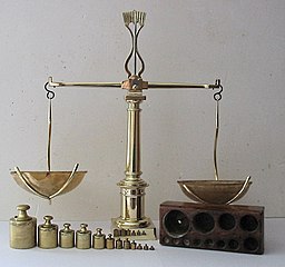
The partition problem has many variations, but recently I encountered it as an interactive puzzle on a computer. (Try a similar game yourself!) The player is presented with an old-fashioned pan-balance scale and a set of objects of different weights. The challenge is to divide (or partition) the objects into two group. You put one group of weights on one side of the scale and the remaining group on the other side so that the scale balances.

Here's a canonical example of the partition problem for two groups. The weights of six items are X = {0.4, 1.0, 1.2, 1.7, 2.6, 2.7}. Divide the objects into two groups of three items so that each group contains half the weight, which is 4.8 for this example. Give it a try! I'll give a solution in the next section.

As is often the case, there are at least two ways to solve this problem: the brute-force approach and an optimization method that minimizes the difference in weights between the two groups. One advantage of the brute-force approach is that it is guaranteed to find all solutions. However, the brute-force method quickly becomes impractical as the number of items increases.

This article considers brute-force solutions. A more elegant solution will be discussed in a future article.

Permutations: A brute-force approach

Let's assume that the problem specifies the number of items that should be placed in each group. One way to specify groups is to use a vector of ±1 values to encode the group to which each item belongs. For example, if there are six items, the vector c = {-1, -1, -1, +1, +1, +1} indicates that the first three items belong to one group and the last three items belong to the other group.

One way to solve the partition problem for two groups is to consider all permutations of the items. For example, Y = {0.4, 1.7, 2.7, 1.0, 1.2, 2.6} is a permutation of the six weights in the previous section. The vector c = {-1, -1, -1, +1, +1, +1} indicates that the items {0.4, 1.7, 2.7} belong to one group and the items {1.0, 1.2, 2.6} belong to the other group. Both groups have 4.8 units of weight, so Y is a solution to the partition problem.

Notice that the inner product Y`*c = 0 for this permutation. Because c is a vector of ±1 values, the inner product is the difference between the sum of weights in the first group and the sum of weights in the second group. An inner product of 0 means that the sums are the same in both groups.

A program to generate all partitions

Let's see how you can use the ALLPERM function in SAS/IML to solve the two-group partition problem. Since the number of permutations grows very fast, let's use an example that contains only four items. The weights of the four items are X = {1.2, 1.7, 2.6, 3.1}. We want two items in each group, so define c = {-1, -1, 1, 1}. We search for a permutation Y = π(X), such that Y`*c = 0. The following SAS/IML program generates ALL permutations of the integers {1,2,3,4}. For each permutation, the sum of the first two weights is compared to the sum of the last two weights. The permutations for which Y`*c = 0 are solutions to the partition problem.

proc iml;
X = {1.2, 1.7, 2.6, 3.1};
c = { -1,  -1,   1,   1};  /* k = 2 */
 
/* Brute Force Method 1: Generate all permutations of items */
N = nrow(X);
P = allperm(N);            /* all permutations of 1:N */
Y = shape( X[P], nrow(P), ncol(P) );   /* reshape to N x N! matrix */
z = Y * c;                 /* want to find z=0 (or could minimize z) */
idx = loc(abs(z) < 1E-8);  /* indices where z=0 in finite precision */
Soln = Y[idx, ];           /* return all solutions; each row is solution */

This program generates P, a matrix whose rows contain all permutations of four elements. The matrix Y is a matrix where each row is a permutation of the weights. Therefore, Y*c is the vector of all differences. When a difference is zero, the two groups contain the same weights. The following statements count how many solutions are found and print the first solution:

numSolns = nrow(soln);
s = soln[1,];
print numSolns, s[c={'L1' 'L2' 'R1' 'R2'}];

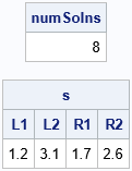
There are a total of eight solutions. One solution is to put the weights {1.2, 3.1} in one group and the weights {1.7, 2.6} in the other group. What are the other solutions? For this set of weights, the other solutions are trivial variations of the first solution. The following statement prints all the solutions:

print soln[c={'L1' 'L2' 'R1' 'R2'}];

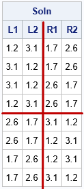
I have augmented the output so that it is easier to see the structure. In the first four rows, the values {1.2, 3.1} are in the first group and the values {1.7, 2.6} are in the second group. In the last four rows, the values switch groups. Thus, this method, which is based on generating all permutations, generates a lot of solutions that are qualitatively the same, in practice.

Combinations: Another brute-force approach

The all-permutation method generates N! possible partitions and, as we have seen, not all the partitions are qualitatively different. Thus, using all permutations is inefficient. A more efficient (but still brute-force) method is to use combinations instead of permutations. Combinations are essentially a sorted version of a permutation. The values {1, 2, 3}, {2, 1, 3}, and {3, 2, 1} are different permutations, whereas there is only one combination ({1, 2, 3}) that contains these three numbers. If there are six items and you want three items in each group, there are 6! = 720 permutations to consider, but only "6 choose 3" = 20 combinations.

The following SAS/IML function uses combinations to implement a brute-force solution of the two-group partition problem. The Partition2_Comb function takes a vector of item weights and a vector (nPart) that contains the number of items that you want in the first and second groups. If you want k items in the first group, the ALLCOMB function creates the complete set of combinations of k indices. The SETDIFF function computes the complementary set of indices. For example, if there are six items and {1, 4, 5} is a set of indices, then {2, 3, 6} is the complementary set of indices. After the various combinations are defined, the equation Y*c = 0 is used to find solutions, if any exist, where the first k elements of c are -1 and the last N-k elements are +1.

/* Brute Force Method 2: Generate all combination of size k, N-k */
start Partition2_Comb(_x, k, tol=1e-8);
   x = colvec(_x);
   N = nrow(x);
   call sort(x);                 /* Optional: standardize the output */
 
   c = j(k, 1, -1) // j(N-k, 1, 1); /* construct +/-1 vector */
   L = allcomb(N, k);            /* "N choose k" possible candidates in "left" group */
   R = j(nrow(L), N-k, .);
   do i = 1 to nrow(L);
      R[i,] = setdif(1:N, L[i,]);  /* complement indices in "right" group */
   end;
   P = L || R;                   /* combine the left and right indices */
 
   Y = shape( X[P], nrow(P) );   /* reshape X[P] into an N x (N choose k) matrix */
   z = Y * c;                    /* want to find z=0 (or could minimize z) */
   solnIdx = loc(abs(z) < tol);  /* indices where z=0 in finite precision */
   if ncol(solnIdx) = 0 then 
      soln = j(1, N, .);         /* no solution */
   else
      soln = Y[solnIdx, ];       /* each row is solution */
   return soln;                  /* return all solutions */
finish;
 
/* test the function on a set that has 11 items, partitioned into groups of 5 and 6 */
x = {0.8, 1.2, 1.3, 1.4, 1.6, 1.8, 1.9, 2.0, 2.2, 2.3, 2.5}; 
soln = Partition2_Comb(x, 5);
numSolns = nrow(soln);
print numSolns, soln[c=(('L1':'L5') || ('R1':'R6'))];

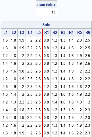
The output shows 13 solutions for a set of 11 items that are partitioned into two groups, one with five items and the other with 11-5=6 items. For the solution, each partition has 9.5 units of weight.

Summary

This article shows some SAS/IML programming techniques for using a brute-force method to solve the partition problem on N items. In the partition problem, you split items into two groups that have k and N-k items so that the weight of the items in each group is equal. This article introduced the solution in terms of all permutations of the items, but implemented a solution in terms of all combinations, which eliminates redundant orderings of the items.

In many applications, you don't need to find all solutions, you just need any solution. A subsequent article will discuss formulating the partition problem as an optimization that seeks to minimize the difference between the weights of the two groups.