I previously wrote about one way to solve the partition problem in SAS. In the partition problem, you divide (or partition) a set of N items into two groups of size k and N-k such that the sum of the items' weights is the same in each group. For example, if the weights of six items are X = {0.4, 1.0, 1.2, 1.7, 2.6, 2.7} and k=3, you can put the weights {0.4, 1.7, 2.7} in one group and the weights {1.0, 1.2, 2.6} in the other group. Both groups contain 4.8 units of weight.

The previous article discussed a brute-force approach in which you explicitly generate all combinations of k items from the set of N items. The program could produce all possible solutions, provided that a solution exists. This article recasts the partition problem as an optimization problem and shows two ways to solve it:

• A feasibility problem: Define the problem as a set of constraints. Find one or more solutions that satisfy the constraints.
• An optimization problem: Find a partition that minimizes the difference between the weights in the two groups. When there is a solution, this method finds it. If there is not a solution, this method finds partitions that distribute the weight as equally as possible.

This article shows how to use PROC OPTMODEL in SAS/OR software. In SAS Viya, you can submit the same statements by using the OPTMODEL procedure in SAS Optimization or the runOptModel action. I thank my colleague, Rob Pratt, who wrote the programs in this article and also kindly reviewed both articles about the partition problem.

A feasible set of binary vectors

The previous article formulated the problem in terms of a binary vector. I defined an N-dimensional vector, c, that contained k elements with the value -1 and N-k elements with the value +1. The two values of the vector c indicate whether an item belongs to the first group or the second group. If X is a solution (an ordering of the weights that satisfied the partition problem), then the inner product X`*c=0.

In this article, it is more convenient to define the two groups by using a 0/1 binary indicator vector, Y. With this definition of Y, a solution satisfies the equation X`*Y = X`*(1-Y). The equation specifies that the sum of weights in the '1' group equals the sum of weights in the '0' group.

To define the feasible set of Y vectors that solve the partition problem, you can define the following two constraints:

1. 1`*Y = k, where 1 is the vector of 1s. This constraint requires that there be exactly k values of Y that are equal to 1.
2. X`*Y = X`*(1-Y). This constraint means that the sum of the k values of X in the first set equals the sum of the N-k values of X in the second set.

The OPTMODEL procedure enables you to specify the problem and the constraints in a natural syntax. Instead of using vector notation, as I did above, it uses summations and indices. The following statements define a set that has 11 items that are to be partitioned into two groups that contain 5 and 6 items, respectively. This program returns an arbitrary feasible point and prints the solution:

/* feasibility problem: enforce equal group weights */
proc optmodel;
set ITEMS = 1..11;
num weight {ITEMS} = [0.8, 1.2, 1.3, 1.4, 1.6, 1.8, 1.9, 2.0, 2.2, 2.3, 2.5];
num k = 5;
 
/* Y[i] = 1 if item i is in group 1; Y[i] = 0 if item i is in group 2 */
var Y {ITEMS} binary;
 
/* group 1 must contain exactly k items */
con NumItemsInGroup1:            /* 1`*Y = k */
   sum{i in ITEMS} Y[i] = k;
 
/* constraint: each group must contain the same weight */
con SameWeightInEachGroup:      /* weight`*Y = weight`*(1-Y) */
   sum{i in ITEMS} weight[i] * Y[i] = sum{i in ITEMS} weight[i] * (1 - Y[i]);
 
/* find one feasible solution */
solve noobj;        /* default solver is MILP */
print Y weight;

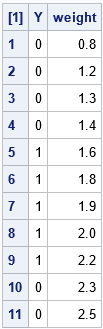
As shown in the output, this solution partitions the weights {1.6, 1.8, 1.9, 2.0, 2.2} into one group and the other six weights into another group.

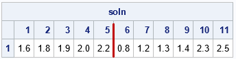
The solution is shown as a column vector. Because we will want to display multiple solutions, it is convenient to transpose the solution (or set of solutions) so that each solution is a row vector in a matrix. It is also helpful to standardize the solution vector so that the left-most k elements contain the items in one group, and the right-most N-k elements contain the elements in the other group. Fortunately, PROC OPTMODEL provides programming statements and the automatic variable _NSOL_, which tells us how many solutions were found. The following macro code fills a matrix that has _NSOL_ rows and N=11 columns. It then puts one group of weights into the first k columns and the other group in the last N-k columns. Because PROC OPTMODEL is an interactive procedure, it does not stop running until you specify a QUIT statement. Therefore, the procedure is still running, and you can submit the following statements:

/* Macro to print table with one row per solution. Put the group 
   with k items on the left and the group with N-k items on the right. */
%macro printSolutionTable;
for {s in 1.._NSOL_} do;
   leftCount  = 0;
   rightCount = 0;
   for {i in ITEMS} do;
      if Y[i].sol[s] > 0.5 then do;
         leftCount = leftCount + 1;
         soln[s,leftCount] = weight[i];
      end;
      else do;
         rightCount = rightCount + 1;
         soln[s,k+rightCount] = weight[i];
      end;
   end;
end;
print soln;
%mend printSolutionTable;
 
/* define the matrix soln and the index variables */
num soln {1.._NSOL_, 1..card(ITEMS)};
num leftCount, rightCount;
%printSolutionTable;

Find all feasible solutions to the partition problem

The previous section found one solution to the partition problem. If you want to find additional solutions, you can add options to the SOLVE statement. The options depend on the solver that you use. The previous SOLVE statement used the MILP solver. You can obtain additional solutions by using the following options:

/* find up to 100 feasible solutions */
solve noobj with milp / maxpoolsols=100 soltype=best;
put _NSOL_=;
%printSolutionTable;

By the way, you can also use constraint logic programming (CLP) to solve this problem. The CLP solver supports the FINDALLSOLNS option, which you can specify as follows:

/* an alternate way to find all feasible solutions */
solve with clp / findallsolns;

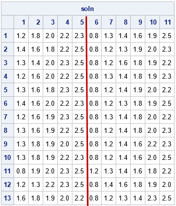
Both methods find all 13 solutions that were found in the previous article.

Minimize the absolute deviations between groups

In the previous sections, the second constraint ensures that the difference between the weights in the two groups is exactly zero. However, you might have data that cannot be evenly divided. In that case, you might want to find a partition that minimizes the absolute deviance between the two groups. You can do that by using the second equation as an objective function rather than as a constraint.

Note that you must minimize the ABSOLUTE VALUE of the difference between the weights in the two groups. If you minimize the difference, the optimization will put the smallest weights in one group and the largest in the other.

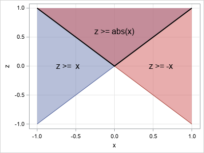
The absolute value of a linear function is not linear. However, you can use a standard trick to rewrite the objective function as a linear function subject to two linear constraints. Let x be the quantity to minimize. Recall that the absolute value |x| is defined by x when x≥0 and by -x when x≤0. Introduce a new variable, z, subject to the linear constraints that z ≥ x and z ≥ -x. The graph at the right shows the geometry of this choice. Minimizing the constrained variable z is equivalent to minimizing |x|, but it can be done by using linear programming techniques. For more information about handling absolute values in the objective function, see this "open textbook" from Cornell University.

By using this trick, you can formulate the partition problem as an optimization that minimizes the absolute deviation between the sum of weights in the two groups:

/* optimization problem: minimize absolute difference of group weights */
proc optmodel;
set ITEMS = 1..11;
num weight {ITEMS} = [0.8, 1.2, 1.3, 1.4, 1.6, 1.8, 1.9, 2.0, 2.2, 2.3, 2.5];
num k = 5;
 
/* Y[i] = 1 if item i is in group 1; Y[i] = 0 if item i is in group 2 */
var Y {ITEMS} binary;
 
/* group 1 must contain exactly k items */
con NumItemsInGroup1:
   sum{i in ITEMS} Y[i] = k;
 
/* minimize absolute difference of group weights */
/* Use a standard trick to handle absolute values in an objective function:
   z=|L*y| is z = {  L*y if L*y >= 0
                  { -L*y if L*y <  0
*/
var AbsValue;
min GroupWeightDifference = AbsValue;
 
con Linearize1:
   AbsValue >=  sum{i in ITEMS} weight[i] * Y[i] - sum{i in ITEMS} weight[i] * (1 - Y[i]);
con Linearize2:
   AbsValue >= -sum{i in ITEMS} weight[i] * Y[i] + sum{i in ITEMS} weight[i] * (1 - Y[i]);
 
/* find up to 100 optimal solutions */
solve with milp / maxpoolsols=100 soltype=best presolver=none;
put _NSOL_=;
 
num soln {1.._NSOL_, 1..card(ITEMS)};
num leftCount, rightCount;
%printSolutionTable;

This optimization also finds the 13 solutions, although the rows are displayed in a different order. The output is not shown.

An advantage of this formulation is that this technique enables you to handle the case where an exact solution is not possible. For example, if you change the smallest weight from 0.8 to 0.85, it is no longer possible to partition the weights evenly. However, the optimization continues to find 13 solutions, only now each solution defines two groups in which the weights differ by 0.05, which is the smallest possible difference.

Easier syntax in SAS Viya

The trick that handles an absolute value in an objective function is one example of a general method that can "linearize" several types of problems. In SAS Viya, there is an automatic way to perform "linearization" for these standard problems. In SAS Optimization software, PROC OPTMODEL supports the LINEARIZE option, beginning in SAS Viya 2020.1.1 (December 2020). Thus, in Viya you can solve the partition problem by using a simpler syntax:

/* show the LINEARIZE option in SAS Viya 2020.1.1 */
min GroupWeightDifference =
   abs( sum{i in ITEMS} weight[i] * Y[i] - sum{i in ITEMS} weight[i] * (1 - Y[i]) );
solve with milp LINEARIZE / maxpoolsols=100 soltype=best;

Summary

This article shows some optimization techniques for solving the partition problem on N items. You can use PROC OPTMODEL in SAS to solve the partition problem in two ways. If the partition problem has a solution, you can formulate the problem as a feasibility problem. Alternatively, you can minimize the absolute deviations between the two groups. This second approach will also find approximate partitions when an exact solution is not possible.

This article also shows a standard trick that enables you to optimize the absolute value of a linear objective function. The trick is to replace the absolute value by using two linear constraints. In SAS Viya, the LINEARIZE option implements the trick automatically.