The number of possible bootstrap samples for a sample of size N is big. Really big.

Recall that the bootstrap method is a powerful way to analyze the variation in a statistic. To implement the standard bootstrap method, you generate B random bootstrap samples. A bootstrap sample is a sample with replacement from the data. The phrase "with replacement" is important. In fact, a bootstrap sample is sometimes called a "resample" because it is generated by sampling the data with REplacement.

This article compares the number of samples that you can draw "with replacement" to the number of samples that you can draw "without replacement." It demonstrates, for very small samples, how to generate the complete set of bootstrap samples. It also explains why generating a complete set is impractical for even moderate-sized samples.

The number of samples with and without replacement

For a sample of size N, there are N! samples if you sample WITHOUT replacement (WOR). The quantity N! grows very quickly as a function of N, so the number of permutations is big for even moderate values of N. In fact, I have shown that if N≥171, then you cannot represent N! by using a double-precision floating-point value because 171! is greater than MACBIG (=1.79769e+308), which is the largest value that can be represented in eight bytes.

However, if you sample WITH replacement (WR), then the number of possible samples is N^N, which grows even faster than the factorial function! If the number of permutations is "big," then the number of WR samples is "really big"!

For comparison, what do you think is the smallest value of N such that N^N exceeds the value of MACBIG? The answer is N=144, which is considerably smaller than 171. The computation is shown at the end of this article.

Another way to compare the relative sizes of N! and N^N is to print a few values of both functions for small values of N. The following table shows the values for N≤10:

proc iml;
N = 1:10;
nPerm = fact(N);     /* N!  */
nResamp = N##N;      /* N^N */
both = nPerm // nResamp;
print both[r={"Permutations" "Samples (WR)"} c=N format=comma15. L=""];

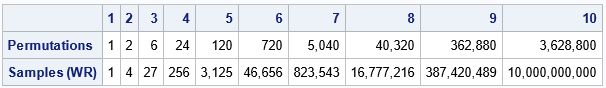
Clearly, the number of bootstrap samples (samples WR) grows very big very fast. This is why the general bootstrap method uses random bootstrap samples rather than attempting some sort of "exact" computation that uses all possible bootstrap samples.

An exact bootstrap computation that uses all possible samples

If you have a VERY small data set, you could, in fact, perform an exact bootstrap computation. For the exact computation, you would generate all possible bootstrap samples, compute the distribution on each sample, and thereby obtain the exact bootstrap distribution of the statistic.

Let's carry out this scheme for a data set that has N=7 observations. From the table, we know that there are exactly 7⁷ = 823,543 samples with replacement.

For small N, it's not hard to construct the complete set of bootstrap samples: just form the Cartesian product of the set with itself N times. In the SAS/IML language, you can use the ExpandGrid function to define the Cartesian product. If the data has 7 values, the Cartesian product will be a matrix that has 823,543 rows and 7 columns.

The following SAS/IML program performs a complete bootstrap analysis of the sample mean. The sample, S, has 7 observations. The minimum value is -1; the maximum value is 4. The sample mean is approximately 0.51. What is the bootstrap distribution of the sample mean? You can form the set of all possible subsamples of size 7, where the elements are resampled from S. You can then compute the mean of every resample and plot the distribution of the means:

proc iml;
S = {-1  -0.1  -0.6  0  0.5  0.8  4};
/* 1. compute original statistic */
m = S[:];          /* = mean(S`) */
print m;
 
/* 2. Generate ALL resamples! */
/* Cartesian product of the elements in S is
   S x S x ... x S
   \------v------/
         N times                              */
z = ExpandGrid(S, S, S, S, S, S, S);
 
/* 3. Compute statistic on each resample */
means = z[,:];
 
/* 4. Analyze the bootstrap distribution */
title "Complete Bootstrap Distribution of the Mean";
title2 "N = 7";
call histogram(means) rebin={-1 0.1} xvalues=-1:4
     other="refline 0.51/axis=x lineattrs=(color=red);";

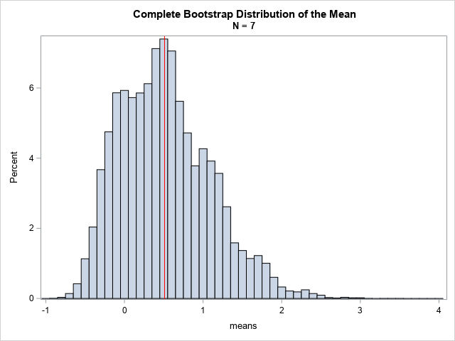
The graph shows the mean for every possible resample of size 7. The mean of the original sample is shown as a red vertical line. Here are some of the resamples in the complete set of bootstrap samples:

• The resamples where a datum is repeated seven times. For example, one resample is {-1, -1, -1, -1, -1, -1, -1}, which has a mean of -1. Another resample is {4, 4, 4, 4, 4, 4, 4}, which has a mean of 4. These two resamples define the minimum and maximum values, respectively, of the bootstrap distribution. There are only seven of these resamples.
• The resamples where a datum is repeated six times. For example, one of the resamples is {-1, -1, -1, -1, -1, -1, 4}. Another is {-1, -1, 0, -1, -1, -1, -1}. A third is {4, 4, 4, 4, 4, 4, 4}, which has a mean of 4. These two resamples define the minimum and maximum values. Another resample is {4, 4, 4, 4, 0.5, 4, 4}. There are 7³ resamples of this type.
• The resamples where each datum is present exactly one time. These sets are all permutations of the sample itself, {-1 -0.1 -0.6 0 0.5 0.8 4}. There are 7! = 5,040 resamples of this type. Each of these permutations has the same mean, which is 0.51. This helps to explain why there is a visible peak in the distribution at the value of the sample mean.

The bootstrap distribution does not make any assumptions about the distribution of the data, nor does it use any asymptotic (large sample) assumptions. It uses only the observed data values.

Comparison with the usual bootstrap method

For larger samples, it is impractical to consider ALL possible samples of size N. Therefore, the usual bootstrap method generates B random samples (with replacement) for a large value of B. The resulting distribution is an approximate bootstrap distribution. The following SAS/IML statements perform the usual bootstrap analysis for B=10,000.

/* Generate B random resamples. Compute and analyze bootstrap distribution */
call randseed(123);
w = sample(S, {7, 10000});   /* 10,000 samples of size 7 (with replacement) */
means = w[,:];
title "Bootstrap Distribution of the Mean";
title2 "B = 10,000; N = 7";
call histogram(means) rebin={-1 0.1} xvalues=-1:4
     other="refline 0.51/axis=x lineattrs=(color=red);";

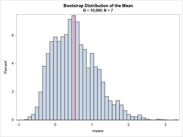
The resulting bootstrap distribution is similar in shape to the complete distribution, but only uses 10,0000 random samples instead of all possible samples. You can see that the properties of the second distribution (such as quantiles) will be similar to the quantiles of the complete distribution, even though the second distribution is based on many fewer bootstrap samples.

Summary

For a sample of size N, there are N^N possible resamples of size N when you sample with replacement. The bootstrap distribution is based on a random sample of these resamples. When N is small, you can compute the exact bootstrap distribution by forming the Cartesian product of the sample with itself N times. This article computes the exact bootstrap distribution for the mean of seven observations and compares the exact distribution to an approximate distribution that is based on B random resamples. When B is large, the approximate distribution looks similar to the complete distribution.

For more about the bootstrap method and how to perform bootstrap analyses in SAS, see "The essential guide to bootstrapping in SAS."

Appendix: Solving the equation N^N = y

This article asked, "what is the smallest value of N such that N^N exceeds the value of MACBIG?" The claim is that N=144, but how can you prove it?

For any value of y > 1, you can use the Lambert W function to find the value of N that satisfies the equation N^N ≤ y. Here's how to solve the equation:

1. Take the natural log of both sides to get N*log(N) ≤ log(y).
2. Define w = log(N) and x = log(y). Then the equation becomes w exp(w) ≤ x. The solution to this equation is found by using the Lambert W function: w = W(x).
3. The solution to the original equation is N = exp(w). Since N is supposed to be an integer, round up or down, according to the application.

The following SAS/IML program solves for the smallest value of N such that N^N exceeds the value of MACBIG in double-precision.

proc iml;
x = constant('LogBig');   /* x = log(MACBIG) */
w = LambertW(x);          /* solve for w such that w*exp(w) = x */
N1 = exp(w);              /* because N = log(w) */
N = ceil(N1);             /* round up so that N^N exceeds MACBIG */
print N1 N;
quit;

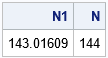
So, when N=144, N^N is larger than the maximum representable double-precision value (MACBIG).