Bootstrap correlation coefficients in SAS

You can use the bootstrap method to estimate confidence intervals. Unlike formulas, which assume that the data are drawn from a specified distribution (usually the normal distribution), the bootstrap method does not assume a distribution for the data. There are many articles about how to use SAS to bootstrap statistics for univariate data and for data from a regression model. This article shows how to bootstrap the correlation coefficients in multivariate data. The main challenge is that the correlation coefficients are typically output in a symmetric matrix. To analyze the bootstrap distribution, you must convert the statistics from a "wide form" (a matrix) to a "long form" (a column), as described in a previous article.

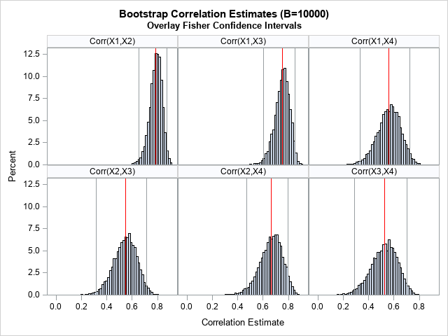
To motivate the bootstrap method for correlations, recall that PROC CORR in SAS supports the FISHER option, which estimates confidence intervals for the correlation coefficients. However, the interval estimates are parametric: they assume that the pairs of variables are bivariate normal. How good are the estimates for real data? You can generate the bootstrap distribution for the correlation coefficients and compare the Fisher confidence intervals to the bootstrap estimates. As a preview of things to come, the graph to the right (click to expand) shows histograms of bootstrap estimates and the Fisher confidence intervals.

This article assumes that the reader is familiar with basic bootstrapping in SAS. If not, see the article, "Compute a bootstrap confidence interval in SAS."

Bootstrap multivariate data in SAS

The basic steps of the bootstrap algorithm are as follows:

Compute a statistic for the original data.
Use PROC SURVEYSELECT to resample (with replacement) B times from the data.
Use BY-group processing to compute the statistic of interest on each bootstrap sample.
Use the bootstrap distribution to obtain estimates of bias and uncertainty, such as confidence intervals.

Let's use a subset of Fisher's Iris data for this example. There are four variables to analyze, so you have to estimate confidence intervals for 4*3/2 = 6 correlation coefficients. For this example, let's use the FISHER option to estimate the confidence intervals. We can then compute the proportion of bootstrap estimates that fall within those confidence intervals, thereby estimating the coverage probability of the Fisher intervals? Does a 95% Fisher interval have 95% coverage for these data? Let's find out!

Step 1: Compute statistics on the original data

The following SAS statements subset the Sashelp.Iris data and call PROC CORR to estimate Fisher's confidence intervals for the six correlation coefficients:

data sample;   /* N = 50 */
   set Sashelp.Iris(where=(Species="Versicolor"));
   label PetalLength= PetalWidth= SepalLength= SepalWidth=;
run;
 
/* STEP 1: Compute statistics on the original data */
%let varNames = PetalLength PetalWidth SepalLength SepalWidth;
%let numVars=4;
proc corr data=sample fisher(biasadj=no) noprob plots=matrix;
   var &varNames;
   ods output FisherPearsonCorr=FPCorr(keep=Var WithVar NObs Corr Lcl Ucl);
run;
 
proc print data=FPCorr noobs; run;

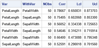
The output shows the estimates for the 95% Fisher confidence intervals for the correlation coefficients. Remember, these estimates assume bivariate normality. Let's generate a bootstrap distribution for the correlation statistics and examine how well the Fisher intervals capture the sampling variation among the bootstrap estimates.

Steps 2 and 3: Bootstrap samples and the bootstrap distribution

As shown in other articles, you can use PROC SURVEYSELECT in SAS to generate B bootstrap samples of the data. Each "bootstrap sample" is a sample (with replacement) from the original data. You can then use the BY statement in PROC CORR to obtain B correlation matrices, each estimated from one of the bootstrap samples:

/* STEP 2: Create B=10,000 bootstrap samples */
/* Bootstrap samples */
%let NumSamples = 10000;       /* number of bootstrap resamples */
proc surveyselect data=sample NOPRINT seed=12345
     out=BootSamples
     method=urs              /* resample with replacement */
     samprate=1              /* each bootstrap sample has N observations */
     /* OUTHITS                 option to suppress the frequency var */
     reps=&NumSamples;       /* generate NumSamples bootstrap resamples */
run;
 
/* STEP 3. Compute the statistic for each bootstrap sample */
proc corr data=BootSamples noprint outp=CorrOut;
   by Replicate;
   freq NumberHits;
   var &varNames;
run;

For many bootstrap analyses, you can proceed directly to the next step, which is to summarize the bootstrap distribution. However, in this case, the statistics in the CorrOut data set are not in a convenient format. The statistics are stored in matrices, as shown by the following call to PROC PRINT, which prints the correlation estimates for the first two bootstrap samples:

/* look at estimates for first two bootstrap samples */
proc print data=CorrOut noobs;
   where _Type_="CORR" & Replicate<=2;
run;

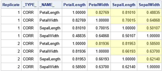
To analyze the distribution of the correlation estimates, it is useful to reshape the data, as described in a previous article. The article shows how to obtain only the values in the cells that are highlighted in yellow. The article also shows how to add labels that identify the pairs of variables. The following DATA step reshapes the data and adds labels such as "Corr(X1,X2)":

/* Convert correlations in the OUTP= data set from wide to long form. See
   https://blogs.sas.com/content/iml/2021/08/25/symmetric-matrix-wide-to-long.html */
data BootLong;
set CorrOut(where=(_Type_="CORR") rename=(_NAME_=Var1));
length Var2 $32 Label $13;
array X[*] &varNames;
Row = 1 + mod(_N_-1, &NumVars);
do Col = Row+1 to &NumVars;       /* names for columns */
   Var2 = vname(X[Col]);
   Corr = X[Col];
   Label = cats("Corr(X",Row,",X",Col,")");
   output;
end;
drop _TYPE_ &varNames;
run;

The bootstrap estimates are now in a "long format," which makes it easier to analyze and visualize the bootstrap distribution of the estimates.

The next section combines the original estimates and the bootstrap estimates. To facilitate combining the data sets, you need to add the Label column to the data set that contains the Fisher intervals. This was also described in the previous article. Having a common Label variable enables you to merge the two data sets.

/* add labels to the Fisher statistics */
data FisherCorr;
length Label $13;
set FPCorr;
retain row col 1;
if col>=&NumVars then do; row+1; col=row; end;
col+1;
Label = cats("Corr(X",row,",X",col,")");
run;

Step 4: Analyze the bootstrap distribution

You can graph the bootstrap distribution for each pair of variables by using the SGPANEL procedure. The following statements create a basic panel:

proc sgpanel data=BootLong;
   panelby Label;
   histogram Corr;
run;

However, a goal of this analysis is to compare the Fisher confidence intervals (CIs) to the bootstrap distribution of the correlation estimates. Therefore, it would be nice to overlay the original correlation estimates and Fisher intervals on the histograms of the bootstrap distributions. To do that, you can concatenate the BootLong and the FisherCorr data sets, as follows:

/* STEP 4: Analyze the bootstrap distribution */
/* overlay the original sample estimates and the Fisher confidence intervals */
data BootLongCI;
set BootLong FisherCorr(rename=(Var=Var1 WithVar=Var2 Corr=Estimate));
label Corr="Correlation Estimate";
run;
 
title "Bootstrap Correlation Estimates (B=&NumSamples)";
title2 "Overlay Fisher Confidence Intervals";
proc sgpanel data=BootLongCI;
   panelby Label / novarname;
   histogram Corr;
   refline Estimate / axis=X lineattrs=(color=red);
   refline LCL / axis=X ;
   refline UCL / axis=X ;
run;

The graph is shown at the top of this article. In the graph, the red lines indicate the original estimates of correlation from the data. The gray vertical lines show the Fisher CIs for the data. The histograms show the distribution of the correlation estimates on 10,000 bootstrap re-samples of the data.

Visually, it looks like the Fisher confidence intervals do a good job of estimating the variation in the correlation estimates. It looks like most of the bootstrap estimates are contained in the 95% CIs.

The coverage of Fisher's confidence intervals

You can use the bootstrap estimates to compute the empirical coverage probability of the Fisher CIs. That is, for each pair of variables, what proportion of the bootstrap estimates (out of 10,000) are within the Fisher intervals? If all pairs of variables were bivariate normal, the expected proportion would be 95%.

You can use the logical expression (Corr>=LCL & Corr<=UCL) to create a binary indicator variable. The proportion of 1s for this variable equals the proportion of bootstrap estimates that are inside a Fisher interval. The following DATA step creates the indicator variable and the call to PROC FREQ counts the proportion of bootstrap estimates that are in the Fisher interval.

/* how many bootstrap estimates are inside a Fisher interval? */
proc sort data=BootLong; by Label; run;
 
data Pctl;
merge BootLong FisherCorr(rename=(Corr=Estimate));
by Label;
label Corr="Correlation Estimate";
InLimits = (Corr>=LCL & Corr<=UCL);
run;
 
proc freq data=Pctl noprint;
   by Label;
   tables InLimits / nocum binomial(level='1');
   output out=Est binomial;
run;
proc print data=Est noobs;
   var Label N _BIN_ L_BIN U_BIN;
run;

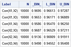
The table shows empirical estimates for the coverage probability of the Fisher intervals. The _BIN_ column contains estimates of the binary proportion. The L_BIN and U_BIN columns contain confidence intervals for the proportions. You can see that all intervals include more than 90% of the bootstrap estimates, and some are close to 95% coverage. The following graph visualizes the empirical coverage for each pair of variables:

ods graphics / width=400px height=240px;
title "Proportion of Bootstrap Estimates in Fisher Intervals"; 
proc sgplot data=Est noautolegend;
   scatter x=_BIN_ y=Label / xerrorlower=L_Bin xerrorupper=U_Bin;
   refline 0.95 / axis=x;
   xaxis  max=1 grid;
   yaxis grid display=(nolabel) offsetmin=0.1 offsetmax=0.1;
run;

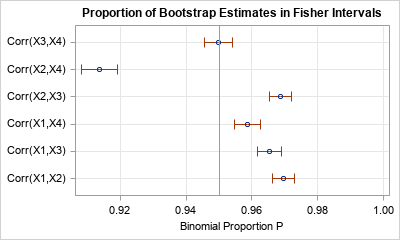
The graph indicates that the many Fisher intervals are too wide (too conservative). Their empirical coverage is greater than the 95% coverage that you would expect for bivariate normal data. On the other hand, the Fisher interval for Corr(X2,X4) has lower coverage than expected.

Summary

This article shows how to perform a bootstrap analysis for correlation among multiple variables. The process of resampling the data (PROC SURVEYSELECT) and generating the bootstrap estimates (PROC CORR with a BY statement) is straightforward. However, to analyze the bootstrap distributions, you need to restructure the statistics by converting the output data from a wide form to a long form. You can use this technique to perform your own bootstrap analysis of correlation coefficients.

Part of the analysis also used the bootstrap distributions to estimate the coverage probability of the Fisher confidence intervals for these data. The Fisher intervals have 95% coverage for normally distributed data. For the iris data, most of the intervals have coverage that is greater than expected, although one interval has lower-than-expected coverage. These results are strongly dependent on the data.

Blogs