Last month a SAS programmer asked how to fit a multivariate Gaussian mixture model in SAS. For univariate data, you can use the FMM Procedure, which fits a large variety of finite mixture models. If your company is using SAS Viya, you can use the MBC or GMM procedures, which perform model-based clustering (PROC MBC) or cluster analysis by using the Gaussian mixture model (PROC GMM). The MBC procedure is part of SAS Visual Statistics; The GMM procedure is part of SAS Visual Data Mining and Machine Learning (VDMML).
Unfortunately, the programmer did not yet have access to SAS Viya. He asked whether you can fit a Gaussian mixture model in PROC IML. Yes, and there are several methods and models that you can fit. Most methods use the expectation-maximization (EM) algorithm. In my opinion, the the Wikipedia entry for the EM algorithm (which includes a Gaussian mixture example) is rather dense. To keep this article as simple as possible, I choose to fit a Gaussian mixture model by using one particular model (full-matrix covariance) and by using a technique called "hard clustering." This article is inspired by a presentation and paper on PROC MBC by Dave Kessler at the 2019 SAS Global Forum. Dave also kindly provided some sample code for me to look at when I was learning about the EM algorithm.
The problem: Fitting a Gaussian mixture model
A Gaussian mixture model assumes that each cluster is multivariate normal but allows different clusters to have different within-cluster covariance structures. As in k-means clustering, it is assumed that you know the number of clusters, G. The clustering problem is an "unsupervised" machine learning problem, which means that the observations do not initially have labels that tell you which observation belongs to which cluster. The goal of the analysis is to assign each observation to a cluster ("hard clustering") or a probability of belonging to each cluster ("fuzzy clustering"). I will use the terms "cluster" and "group" interchangeably. In this article, I will only discuss the hard-clustering problem, which is conceptually easier to understand and implement.
The density of a Gaussian mixture with G components is \(\Sigma_{i=1}^G \tau_i f(\mathbf{x}; {\boldsymbol\mu}_i, {\boldsymbol\Sigma}_i)\), where f(x; μi, Σi) is the multivariate normal density of the i_th component, which has mean vector μi and covariance matrix Σi. The values τi are the mixing probabilities, so Σ τi = 1. If x is a d-dimensional vector, you need to estimate τi, μi, and Σi for each of the G groups, for a total of G*(1 + d + d*(d+1)/2) – 1 parameter estimates. The d*(d+1)/2 expression is the number of free parameters in the symmetric covariance matrix and the -1 term reflects the constraint Σ τi = 1. Fortunately, the assumption that the groups are multivariate normal enables you to compute the maximum likelihood estimates directly without doing any numerical optimization.
Fitting a Gaussian mixture model is a "chicken-and-egg" problem because it consists of two subproblems, each of which is easy to solve if you know the answer to the other problem:
- If you know to which group each observation belongs, you can compute maximum likelihood estimates for the mean (center) and covariance of each group. You can also use the number of observations in each group to estimate the mixing probabilities for the finite mixture distribution.
- If you know the center, covariance matrix, and mixing probabilities for each of the G groups, you can use the density function for each group (weighted by the mixing probability) to determine how likely each observation is to belong to a cluster. For "hard clustering," you assign the observation to the cluster that gives the highest likelihood.
The expectation-maximization (EM) algorithm is an iterative method that enables you to solve interconnected problems like this. The steps of the EM algorithm are given in the documentation for the MBC procedure, as follows:
- Use some method (such as k-means clustering) to assign each observation to a cluster. The assignment does not have to be precise because it will be refined. Some data scientists use random assignment as a quick-and-dirty way to initially assign points to clusters, but for hard clustering this can lead to less than optimal solutions.
- The M Step: Assume that the current assignment to clusters is correct. Compute the maximum likelihood estimates of the within-cluster count, mean, and covariance. From the counts, estimate the mixing probabilities. I have previously shown how to compute the within-group parameter estimates
- The E Step: Assume the within-cluster statistics are correct. I have previously shown how to evaluate the likelihood that each observation belongs to each cluster. Use the likelihoods to update the assignment to clusters. For hard clustering, this means choosing the cluster for which the density (weighted by the mixing probabilities) is greatest.
- Evaluate the mixture log likelihood, which is an overall measure of the goodness of fit. If the log likelihood has barely changed from the previous iteration, assume that the EM algorithm has converged. Otherwise, go to the M step and repeat until convergence. The documentation for PROC MBC provides the log-likelihood function for both hard and fuzzy clustering.
This implementation of the EM algorithm performs the M-step before the E-step, but it is still the "EM" algorithm. (Why? Because there is no "ME" in statistics!)
Use k-means clustering to assign the initial group membership
The first step is to assign each observation to a cluster. Let's use the Fisher Iris data, which we know has three clusters. We will not use the Species variable in any way, but merely treat the data as four-dimensional unlabeled data.
The following steps are adapted from the Getting Started example in PROC FASTCLUS. The call to PROC STDIZE standardizes the data and the call to PROC FASTCLUS performs k-means clustering and saves the clusters to an output data set.
/* standardize and use k-means clustering (k=3) for initial guess */ proc stdize data=Sashelp.Iris out=StdIris method=std; var Sepal: Petal:; run; proc fastclus data=StdIris out=Clust maxclusters=3 maxiter=100 random=123; var Sepal: Petal:; run; data Iris; merge Sashelp.Iris Clust(keep=Cluster); /* for consistency with the Species order, remap the cluster numbers */ if Cluster=1 then Cluster=2; else if Cluster=2 then Cluster=1; run; title "k-Means Clustering of Iris Data"; proc sgplot data=Iris; ellipse x=PetalWidth y=SepalWidth / group=Cluster; scatter x=PetalWidth y=SepalWidth / group=Cluster transparency=0.2 markerattrs=(symbol=CircleFilled size=10) jitter; xaxis grid; yaxis grid; run; |
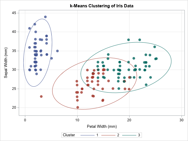
The graph shows the cluster assignments from PROC FASTCLUS. They are similar but not identical to the actual groups of the Species variable. In the next section, these cluster assignments are used to initialize the EM algorithm.
The EM algorithm for hard clustering
You can write a SAS/IML program that implements the EM algorithm for hard clustering. The M step uses the MLEstMVN function (described in a previous article) to compute the maximum likelihood estimates within clusters. The E step uses the LogPdfMVN function (described in a previous article) to compute the log-PDF for each cluster (assuming MVN).
proc iml; load module=(LogPdfMVN MLEstMVN); /* you need to STORE these modules */ /* 1. Read data. Initialize 'Cluster' assignments from PROC FASTCLUS */ use Iris; varNames = {'SepalLength' 'SepalWidth' 'PetalLength' 'PetalWidth'}; read all var varNames into X; read all var {'Cluster'} into Group; /* from PROC FASTCLUS */ close; nobs = nrow(X); d = ncol(X); G = ncol(unique(Group)); prevCDLL = -constant('BIG'); /* set to large negative number */ converged = 0; /* iterate until converged=1 */ eps = 1e-5; /* convergence criterion */ iterHist = j(100, 3, .); /* monitor EM iteration */ LL = J(nobs, G, 0); /* store the LL for each group */ /* EM algorithm: Solve the M and E subproblems until convergence */ do nIter = 1 to 100 while(^converged); /* 2. M Step: Given groups, find MLE for n, mean, and cov within each group */ L = MLEstMVN(X, Group); /* function returns a list */ ns = L$'n'; tau = ns / sum(ns); means = L$'mean'; covs = L$'cov'; /* 3. E Step: Given MLE estimates, compute the LL for membership in each group. Use LL to update group membership. */ do k = 1 to G; LL[ ,k] = log(tau[k]) + LogPDFMVN(X, means[k,], shape(covs[k,],d)); end; Group = LL[ ,<:>]; /* predicted group has maximum LL */ /* 4. The complete data LL is the sum of log(tau[k]*PDF[,k]). For "hard" clustering, Z matrix is 0/1 indicator matrix. DESIGN function: https://blogs.sas.com/content/iml/2016/03/02/dummy-variables-sasiml.html */ Z = design(Group); /* get dummy variables for Group */ CDLL = sum(Z # LL); /* sum of LL weighted by group membership */ /* compute the relative change in CD LL. Has algorithm converged? */ relDiff = abs( (prevCDLL-CDLL) / prevCDLL ); converged = ( relDiff < eps ); /* monitor convergence; if no convergence, iterate */ prevCDLL = CDLL; iterHist[nIter,] = nIter || CDLL || relDiff; end; /* remove unused rows and print EM iteration history */ iterHist = iterHist[ loc(iterHist[,2]^=.), ]; print iterHist[c={'Iter' 'CD LL' 'relDiff'}]; |
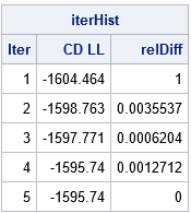
The output from the iteration history shows that the EM algorithm converged in five iterations. At each step of the iteration, the log likelihood increased, which shows that the fit of the Gaussian mixture model improved at each iteration. This is one of the features of the EM algorithm: the likelihood always increases on successive steps.
The results of the EM algorithm for fitting a Gaussian mixture model
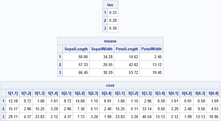
This problem uses G=3 clusters and d=4 dimensions, so there are 3*(1 + 4 + 4*5/2) – 1 = 44 parameter estimates! Most of those parameters are the elements of the three symmetric 4 x 4 covariance matrices. The following statements print the estimates of the mixing probabilities, the mean vector, and the covariance matrices for each cluster. To save space, the covariance matrices are flattened into a 16-element row vector.
/* print final parameter estimates for Gaussian mixture */ GroupNames = strip(char(1:G)); rows = repeat(T(1:d), 1, d); cols = repeat(1:d, d, 1); SNames = compress('S[' + char(rows) + ',' + char(cols) + ']'); print tau[r=GroupNames F=6.2], means[r=GroupNames c=varNames F=6.2], covs[r=GroupNames c=(rowvec(SNames)) F=6.2]; |
You can merge the final Group assignment with the data and create scatter plots that show the group assignment. One of the scatter plots is shown below:
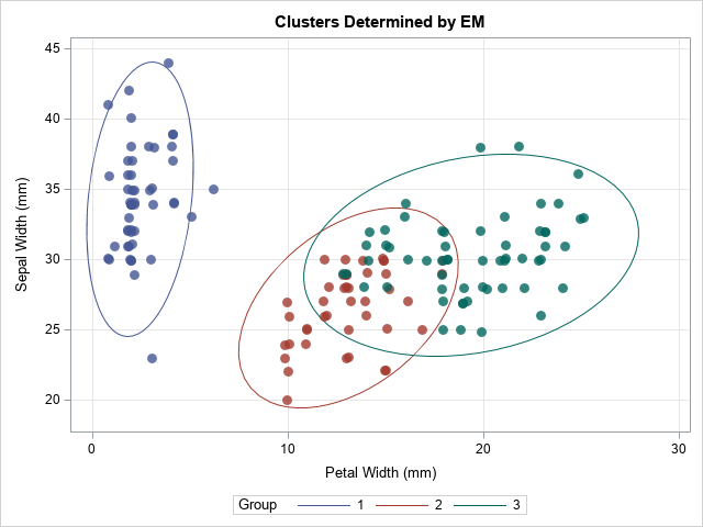
The EM algorithm changed the group assignments for 10 observations. The most obvious change is the outlying marker in the lower-left corner, which changed from Group=2 to Group=1. The other markers that changed are near the overlapping region between Group=2 and Group=3.
Summary
This article shows an implementation of the EM algorithm for fitting a Gaussian mixture model. For simplicity, I implemented an algorithm that uses hard clustering (the complete data likelihood model). This algorithm might not perform well with a random initial assignment of clusters, so I used the results of k-means clustering (PROC FASTCLUS) to initialize the algorithm. Hopefully, some of the tricks and techniques in this implementation of the EM algorithm will be useful to SAS programmers who want to write more sophisticated EM programs.
The main purpose of this article is to demonstrate how to implement the EM algorithm in SAS/IML. As a reminder, if you want to fit a Gaussian mixture model in SAS, you can use PROC MBC or PROC GMM in SAS Viya. The MBC procedure is especially powerful: in Visual Statistics 8.5 you can choose from 17 different ways to model the covariance structure in the clusters. The MBC procedure also supports several ways to initialize the group assignments and supports both hard and fuzzy clustering. For more about the MBC procedure, see Kessler (2019), "Introducing the MBC Procedure for Model-Based Clustering."
I learned a lot by writing this program, so I hope it is helpful. You can download the complete SAS program that implements the EM algorithm for fitting a Gaussian mixture model. Leave a comment if you find it useful.

11 Comments
Rick,
Thank you for presenting this EM algorithm. I wanted to see if I could implement ML estimation of the multivariate Gaussian mixture employing the NLMIXED procedure. What follows is the first post of at least two describing my efforts. Like you, I find this an interesting problem. For ease of presentation, I start out with a bivariate Guassian mixture and build from there.
The bivariate Gaussian model is relatively easy to estimate. We need to compute the log-likelihood for each cluster. You present the log-likelihood of the multivariate Gaussian problem as a function of the log of the determinant of the covariance matrix, the Mahalanobis distance (X-mu)' * inv(V) * (X-mu), and the constant k*log(2*pi) where k is the number of columns in X. For the bivariate model (k=2) with no clustering and V constructed as
_ _
V = | s11 s12 |
| s21 s22 |
-- --
the determinant is Det = s11*s22 - s12*s21. Of course, for a covariance matrix, s21=s12, so we have Det = s11*s22 - s12**2. For a covariance matrix with dimension k=2, the inverse of the covariance matrix is
_ _ _ _
inv(V) = Det**(-1) * | s22 -s21 | = Det**(-1) * | s22 -s12 |
| -s12 s11 | | -s12 s11 |
-- -- -- --
With parameters of the covariance matrix s11, s12, and s22, we can compute Det and Vinv11, Vinv12, and Vinv22 as
Det = s11*s22 - s12**2;
Vinv11 = s22 / Det;
Vinv12 = -s12 / Det;
Vinv22 = s22 / Det;
Then, with parameters mu1 and mu2 for variables X1 and X2, the Mahalanobis distance and log likelihood are computed as
MahalanobisD = ((X1-mu1)**2)*Vinv11 + 2*(X1-mu1)*(X2-mu2)*Vinv12 + ((X2-mu2)**2)*Vinv22;
ll = -0.5 * (log(Det) + MahalanobisD + 2*log(2*constant('pi')));
We can extend the bivariate model to accommodate clustering by having cluster-specific means, variances, determinants, inverses, Mahalanobis distances, and log-likelihoods. We must also introduce the probability that a likelihood contribution belongs to each cluster. The complete log-likelihood function can then be expressed as LL = log( Sum over clusters of exp( log(cluster Prob) * (cluster ll)) ). For a model with three clusters, the complete log-likelihood computation is: LL = log( exp(log(p_c1) + ll_c1) + exp(log(p_c2) + ll_c2) + exp(log(p_c3) + ll_c3) ); The following NLMIXED code estimates a bivariate Gaussian three cluster model with predictors PetalWidth and SepalWidth.
title "Bivariate normal, model with three clusters";
proc nlmixed data=sashelp.iris;
parms mu1_c1 2 mu2_c1 34 /* initialize means for each cluster */
mu1_c2 12 mu2_c2 25
mu1_c3 19 mu2_c3 30
s11_c1 1 s12_c1 1 s22_c1 10 /* initialize covariance for each cluster */
s11_c2 5 s12_c2 1 s22_c2 10
s11_c3 5 s12_c3 1 s22_c3 10
p_c1 p_c2 %sysevalf(1/3); /* initialize cluster probabilities to p_c1=1/3, p_c2=1/3, p3=1/3 */
/* Compute determinant and inverse of cluster 1 variance matrix */
/* Subsequently, compute Mahalanobis distance and log-likelihood for cluster 1 */
Det_c1 = S11_c1*S22_c1 - S12_c1**2;
Vinv11_c1 = S22_c1 / Det_c1;
Vinv12_c1 = -S12_c1 / Det_c1;
Vinv22_c1 = S11_c1 / Det_c1;
MahalanobisD_c1 = ((PetalWidth-mu1_c1)**2)*Vinv11_c1 +
2*(PetalWidth-mu1_c1)*(SepalWidth-mu2_c1)*Vinv12_c1 +
((SepalWidth-mu2_c1)**2)*Vinv22_c1;
ll_c1 = -0.5*(log(Det_c1) + MahalanobisD_c1 + 2*log(2*constant('pi')));
/* Similar computations for cluster 2 */
Det_c2 = S11_c2*S22_c2 - S12_c2**2;
Vinv11_c2 = S22_c2 / Det_c2;
Vinv12_c2 = -S12_c2 / Det_c2;
Vinv22_c2 = S11_c2 / Det_c2;
MahalanobisD_c2 = ((PetalWidth-mu1_c2)**2)*Vinv11_c2 +
2*(PetalWidth-mu1_c2)*(SepalWidth-mu2_c2)*Vinv12_c2 +
((SepalWidth-mu2_c2)**2)*Vinv22_c2;
ll_c2 = -0.5*(log(Det_c2) + MahalanobisD_c2 + 2*log(2*constant('pi')));
/* Similar computations for cluster 3 */
Det_c3 = S11_c3*S22_c3 - S12_c3**2;
Vinv11_c3 = S22_c3 / Det_c3;
Vinv12_c3 = -S12_c3 / Det_c3;
Vinv22_c3 = S11_c3 / Det_c3;
MahalanobisD_c3 = ((PetalWidth-mu1_c3)**2)*Vinv11_c3 +
2*(PetalWidth-mu1_c3)*(SepalWidth-mu2_c3)*Vinv12_c3 +
((SepalWidth-mu2_c3)**2)*Vinv22_c3;
ll_c3 = -0.5*(log(Det_c3) + MahalanobisD_c3 + 2*log(2*constant('pi')));
p_c3 = 1 - p_c1 - p_c2;
/* Compute overall model log-likelihood */
LL = log(exp(log(p_c1) + ll_c1) + exp(log(p_c2) + ll_c2) + exp(log(p_c3) + ll_c3));
/* Estimate model parameters */
model ll ~ general(ll);
/* Generate cluster probabilities for each observation */
predict p_c1*exp(LL_c1)/exp(LL) out=P_c1_BVN_PetalWSepalW;
predict p_c2*exp(LL_c2)/exp(LL) out=P_c2_BVN_PetalWSepalW;
predict p_c3*exp(LL_c3)/exp(LL) out=P_c3_BVN_PetalWSepalW;
run;
A couple of comments about the efficiency of NLMIXED are in order here. It should be noted that the value 2*log(2*Pi) is calculated for every observation in every iteration of the likelihood maximization. It would be ideal if this value could be computed once as part of a CONSTANTS statement (or something similar) and then never again computed but referred to as needed. The NLMIXED procedure does not have such capability, so there is considerable waste of time computing the same value over and over for every observation of every iteration. Similarly, the determinant and inverse matrix are (re-)computed for every observation in each likelihood iteration. Variance parameters are updated with each iteration. But for each update, the variance parameters are fixed. Ideally, there would be no need to compute the determinant and inverse for each observation with each iteration and one would pull out determinant computation and inverse computations to an ITER_CONSTANTS statement. But the NLMIXED procedure does not have either a CONSTANTS or ITER_CONSTANTS statement. So, 2*log(2*pi) and all of the determinant and inverse variance calculations are performed far too often. That renders the NLMIXED procedure rather inefficient - at least when one has to code their own likelihood computations. (I'm sure that for predefined likelihood models, SAS has taken care of these considerations. But when coding one's own likelihood, one presently has to deal with these inefficiencies.)
It would be possible to bypass the issue of computing 2*log(2*Pi) by constructing the value of this constant before the NLMIXED procedure is compiled using SAS macro language processing. Before invoking the NLMIXED procedure, we could compute a constant with code:
%let pi=%sysfunc(constant(pi));
%let TwoPi = %sysevalf(2*&pi);
%let log_2Pi = %sysfunc(log(&TwoPi));
%let k_log_2Pi = %sysevalf(2*&log_2Pi);
Subsequently, we could remove the computation k*log(2*Pi) from the NLMIXED procedure and substitute the value &k_log_2Pi which is a constant given to the NLMIXED compiler wherever the value k_log_2Pi is required.
It should also be noted that it is rather easy to write code for the bivariate Gaussian model because the determinant and variance inverse matrices are easily solved. It becomes more difficult to write code for a multivariate Gaussian model. Of course, one could solve algebraically for both the determinant and the inverse matrix for a covariance matrix of specific size. But that becomes increasingly difficult and prone to error writing the computations employing NLMIXED code as the number of variables in the multivariate Gaussian model increases. Thus, it would be desirable to have methods for computing the determinant and the inverse of a matrix of arbitrary dimension. Subsequent posts provide Base SAS code that operates on matrices (two-dimensional arrays) to implement the following matrix operations:
1) construct the Cholesky decomposition (L) of a matrix (upper-triangular matrix)
2) compute the determinant of the variance matrix as the product of the diagonal elements of the Cholesky decomposition
3) construct the transpose of a matrix (particularly, the Cholesky decomposition L yielding L', a lower-triangular matrix)
4) construct the inverse of a LOWER-triangular matrix mimicking operations implemented in the IML statement Vinv = solve(V, I(k)) where k is the dimension of the covariance matrix to invert. In particular, construct inv( L' )
5) transpose inv( L' ) to obtain inv( L }
6) employ matrix multiplication to compute inv(V) = inv( L ) * inv( L' )
7) employ matrix multiplication to compute the Mahalanobis distance
Since the NLMIXED procedure supports arrays and most Base SAS code, the operations described above can be used to write NLMIXED code which solves the more general multivariate Gaussian mixture model.
Always a pleasure to hear from you, Dale. Thanks for your contribution.
Rick,
I promised some data step methods for doing some matrix operations as part of an overall solution for using the NLMIXED procedure to fit the multivariate Gaussian model. These matrix operations enable solving more than the bivariate Gaussian model. As such, below are SAS macros that perform the following matrix operations:
1) matrix multiplication
2) matrix transpose
3) construction of Cholesky decomposition of a symmetric, full rank matrix
4) computation of determinant from Cholesky decomposition
5) inversion of full rank, lower diagonal matrix
Each macro is attached as a separate post.
Dale,
Thanks for your contribution. Unfortunately, the blogging software often strips out indenting and muddles code that contains less-than signs, greater-than signs, and ampersands, because these are interpreted as HTML. A code-oriented site such as GitHub or SAS Support Communities provides better support for posting long programs. I'll try to reformat the code you posted.
%macro mat_mult(left=, right=, result=);
/***************************************************************************/
/* This macro multiplies two matrices and returns the result in a matrix */
/* Macro mat_mult operates in a SAS data step. Matrices RESULT, LEFT, */
/* and RIGHT must already be declared in the data step where this macro is */
/* invoked. Furthermore, it is up to the user to ensure that the matrices */
/* are conformable: that the number of columns of LEFT is the same as the */
/* number of rows of RIGHT and that the RESULT matrix has the same number */
/* of rows as LEFT and the same number of columns as RIGHT. */
/* */
/* Macro variables: */
/* Left - the left-side matrix that is multiplied by Right to produce */
/* the Result matrix. Left and Right must conform. That is, */
/* the number of columns of matrix Left must match the number */
/* of rows of matrix Right. */
/* Right - the right-side matrix. (See notes about macro variable Left)*/
/* Result - the matrix that is the product of Left x Right. Dimension */
/* of the Result matrix is determined as the number of rows in */
/* Left and the number of columns in Right. */
/* */
/* Author: Dale McLerran */
/* Fred Hutchinson Cancer Res Ctr */
/* */
/***************************************************************************/
_n_nrowL = dim(&left,1);
_n_ncolL = dim(&left,2);
_n_nrowR = dim(&right,1);
_n_ncolR = dim(&right,2);
do _row=1 to _n_nrowL;
do _col=1 to _n_ncolR;
__sum=0;
do _i_j=1 to _n_ncolL;
__sum + &left[_row, _i_j] * &right[_i_j, _col];
end;
&result[_row, _col] = __sum;
end;
end;
%mend mat_mult;
%macro mat_transpose(input=, transpose=);
/********************************************************/
/* This macro computes the transpose of a matrix */
/* */
/* Arguments: */
/* INPUT - name of a matrix to be transposed */
/* TRANSPOSE - transposed matrix name */
/* */
/* Author: Dale McLerran */
/* Fred Hutchinson Cancer Research Center */
/* */
/********************************************************/
_n_rows = dim(&input,1);
_n_cols = dim(&input,2);
do _i_row=1 to _n_rows;
do _i_col=1 to _n_cols;
&transpose{_i_col,_i_row} = &input{_i_row,_i_col};
end;
end;
%mend;
%macro mat_chol(input=, cholesky=);
/**********************************************************************/
/* This macro computes the Cholesky decomposition for a square matrix */
/* */
/* Macro variables: */
/* input - the matrix that is to be inverted */
/* cholesky - cholesky decomposition of the matrix to be inverted */
/* */
/* Author: Dale McLerran */
/* Fred Hutchinson Cancer Research Center */
/* email: dmclerra@fhcrc.org */
/* */
/**********************************************************************/
_n_dim = dim(&input,1);
/* Initialize to 0 */
do i=1 to _n_dim;
do j=1 to _n_dim;
&cholesky{i,j} = 0;
end;
end;
do j=1 to _n_dim;
do i=1 to j-1;
tmp_sum = 0;
do k=1 to i-1;
tmp_sum + &cholesky{k,i}*&cholesky{k,j};
end;
&cholesky{i,j} = (&input{i,j} - tmp_sum) / &cholesky{i,i};
&cholesky{j,i} = &cholesky{i,j} * 0;
end;
tmp_sum = 0;
do k=1 to j-1;
tmp_sum + &cholesky{k,j}**2;
end;
&cholesky{j,j} = sqrt(&input{j,j} - tmp_sum);
end;
%mend;
%macro mat_det_chol(cholesky=, det=);
/*********************************************************************/
/* Having computed the Cholesky decomposition of a square, symmetric */
/* matrix, this macro then computes the determinant of the Cholesky */
/* matrix. The square of the Cholesky matrix determinant is the */
/* determinant of the matrix which was subjected to Cholesky */
/* decomposition. This macro takes as input the Cholesky matrix */
/* which is the Cholesky decomposition and returns the determinant */
/* not of the Cholesky decomposition but of the matrix which was */
/* subjected to a Cholesky decomposition. Thus, this macro returns */
/* the determinant of the square, symmetric matrix. */
/* */
/* Author: Dale McLerran */
/* Fred Hutchinson Cancer Research Center */
/* */
/*********************************************************************/
_n_dim = dim(&cholesky,1);
&det = 1;
do _irc=1 to _n_dim;
&det = &det*&cholesky[_irc,_irc];
end;
&det = &det*&det;
%mend mat_det_chol;
%macro mat_LowerDiagInv(LowDiagInput=, LowDiagInv=, dim=);
/**********************************************************************/
/* This macro computes the Cholesky decomposition for a square matrix */
/* Subsequently, the Cholesky decomposition is employed to compute */
/* the inverse of the input matrix. */
/* Note that if the original matrix is not full rank but of rank M, */
/* then the inverse matrix which is computed will be the inverse only */
/* through rows 1:M and columns 1:M such that the submatrix */
/* Cholesky[1:M, 1:M] has rank M. */
/* */
/* Macro variables: */
/* LowDiagInput - lower diagonal (square) matrix to be inverted */
/* LowDiagInv - inverse of LowDiagInput matrix */
/* Dim - number of rows in LowDiagInput */
/* */
/* Author: Dale McLerran */
/* Fred Hutchinson Cancer Research Center */
/* */
/**********************************************************************/
%global ScratchMatLDI;
%if &ScratchMatLDI=. %then
%let ScratchMatLDI = 1;
%else %let ScratchMatLDI = %eval(&ScratchMatLDI + 1);
array _scratch_&ScratchMatLDI {&dim,&dim} _temporary_;
do row=1 to &dim;
do col=1 to &dim;
_scratch_&ScratchMatLDI{row,col} = &LowDiagInput{row,col};
if row=col then &LowDiagInv{row,col} = 1;
else &LowDiagInv{row,col}=0;
end;
end;
do pivot=1 to &dim;
do row=pivot to &dim;
scale = _scratch_&ScratchMatLDI[row,pivot];
if scale>1E-10 then do;
do col=1 to &dim;
_scratch_&ScratchMatLDI{row,col} = _scratch_&ScratchMatLDI{row,col} / scale;
&LowDiagInv{row,col} = &LowDiagInv{row,col} / scale;
end;
if row>pivot then do;
do col=1 to &dim;
_scratch_&ScratchMatLDI{row,col} =
_scratch_&ScratchMatLDI{row,col} - _scratch_&ScratchMatLDI{pivot,col};
&LowDiagInv{row,col} = &LowDiagInv{row,col} - &LowDiagInv{pivot,col};
end;
end;
end;
end;
end;
%mend mat_LowerDiagInv;
With these five macros, the multivariate Gaussian model can be estimated with code as demonstrated below. Note that this is not a Gaussian mixture model. I want to introduce the use of these macros to construct and solve the simpler problem first of just a multivariate Gaussian model. Again, I appeal to the sashelp.iris data.
title "Multivariate (k=4) normal model with one cluster";
proc nlmixed data=sashelp.iris(where=(PetalWidth10));
parms mu1 2 mu2 34 mu3 50 mu4 14
s11 2 s12 s13 s14 .5
s22 20 s23 s24 .5
s33 20 s34 .5
s44 10;
/* List variables assumed to have multivariate Gaussian distribution in array */
array _X_ {4} PetalWidth SepalWidth SepalLength PetalLength;
/* List parameters mu in array and construct row vectors and column vectors (X-mu) and T(X-mu) */
array _mu {4} mu1 mu2 mu3 mu4;
array _XminMu {4,1} _temporary_;
array _XminMuT {1,4} _temporary_;
do i=1 to 4;
_xminMu{i,1} = _x_{i} - _mu{i};
_xminMuT{1,i} = _x_{i} - _mu{i};
end;
/* Construct variance matrix. Note that upper triangular part of variance matrix is filled already. */
array _V {4,4} S11 S12 S13 S14
S21 S22 S23 S24
S31 S32 S33 S34
S41 S42 S43 S44;
/* Complete the lower triangular part of the variance matrix */
S21 = S12;
S31 = S13;
S41 = S14;
S32 = S23;
S42 = S24;
S43 = S34;
/* Define matrices holding the Cholesky decomposition of variance L, transpose of L */
/* inverse of T(L), transpose of inv(T(L)), and inverse of the variance matrix */
array _chol {4,4} _temporary_;
array _cholT {4,4} _temporary_;
array _cholInvT {4,4} _temporary_;
array _cholInv {4,4} _temporary_;
array _Vinv {4,4} _temporary_;
/* Now, compute all of these elements */
%mat_chol(input=_V, cholesky=_chol)
%mat_transpose(input=_chol, transpose=_cholT);
%mat_LowerDiagInv(LowDiagInput=_cholT, LowDiagInv=_cholInvT, dim=4)
%mat_transpose(input=_cholInvT, transpose=_cholInv)
%mat_mult(left=_cholInv, right=_cholInvT, result=_Vinv)
%mat_det_chol(cholesky=_chol, det=det)
/* Compute MahalanobisDSq form T(X-mu)*inv(V)*(X-mu) for the cluster */
array _quadLeft {1,4} _temporary_;
array _MahalanobisDSq {1,1} _temporary_;
%mat_mult(left=_XminMuT, right=_Vinv, result=_quadleft)
%mat_mult(left=_quadleft, right=_XminMu, result=_MahalanobisDSq);
/* Compute log-likelihood for the cluster */
LL = -0.5*(log(Det) + _MahalanobisDSq{1,1} + 4*log(2*constant('pi')));
/* Maximize the log-likelihood */
model LL ~ general(LL);
run;
%macro mat_chol(input=, cholesky=);
/**********************************************************************/
/* This macro computes the Cholesky decomposition for a square matrix */
/* */
/* Macro variables: */
/* input - the matrix that is to be inverted */
/* cholesky - cholesky decomposition of the matrix to be inverted */
/* */
/* Author: Dale McLerran */
/* Fred Hutchinson Cancer Research Center */
/* */
/**********************************************************************/
_n_dim = dim(&input,1);
/* Initialize to 0 */
do i=1 to _n_dim;
do j=1 to _n_dim;
&cholesky{i,j} = 0;
end;
end;
do j=1 to _n_dim;
do i=1 to j-1;
tmp_sum = 0;
do k=1 to i-1;
tmp_sum + &cholesky{k,i}*&cholesky{k,j};
end;
&cholesky{i,j} = (&input{i,j} - tmp_sum) / &cholesky{i,i};
&cholesky{j,i} = &cholesky{i,j} * 0;
end;
tmp_sum = 0;
do k=1 to j-1;
tmp_sum + &cholesky{k,j}**2;
end;
&cholesky{j,j} = sqrt(&input{j,j} - tmp_sum);
end;
%mend;