How to evaluate the multivariate normal log likelihood

The multivariate normal distribution is used frequently in multivariate statistics and machine learning. In many applications, you need to evaluate the log-likelihood function in order to compare how well different models fit the data. The log-likelihood for a vector x is the natural logarithm of the multivariate normal (MVN) density function evaluated at x. A probability density function is usually abbreviated as PDF, so the log-density function is also called a log-PDF. This article discusses how to efficiently evaluate the log-likelihood function and the log-PDF. Examples are provided by using the SAS/IML matrix language.

The multivariate normal PDF

A previous article provides examples of using the LOGPDF function in SAS for univariate distributions. Multivariate distributions are more complicated and are usually written by using matrix-vector notation. The multivariate normal distribution in dimension d has two parameters: A d-dimensional mean vector μ and a d x d covariance matrix Σ. The MVN PDF evaluated at a d-dimensional vector x is
$f(\mathbf{x})= \frac{1}{\sqrt { (2\pi)^d|\boldsymbol \Sigma| } } \exp\left(-\frac{1}{2} (\mathbf{x}-\boldsymbol\mu)^{\rm T} \boldsymbol\Sigma^{-1} ({\mathbf x}-\boldsymbol\mu)\right)$
where |Σ| is the determinant of Σ. I have previously shown how to evaluate the MVN density in the SAS/IML language, and I noted that the argument to the EXP function involves the expression MD(x; μ, Σ)² = (x-μ)^TΣ^-1(x-μ), where MD is the Mahalanobis distance between the point x and the mean vector μ.

Evaluate the MVN log-likelihood function

When you take the natural logarithm of the MVN PDF, the EXP function goes away and the expression becomes the sum of three terms:
$\log(f(\mathbf{x})) = -\frac{1}{2} [ d \log(2\pi) + \log(|\boldsymbol \Sigma|) + {\rm MD}(\mathbf{x}; \boldsymbol\mu, \boldsymbol\Sigma)^2 ]$
The first term in the brackets is easy to evaluate, but the second and third terms appear more daunting. Fortunately, the SAS/IML language provides two functions that simplify the evaluation:

The LOGABSDET function computes the logarithm of the absolute value of the determinant of a matrix. For a full-rank covariance matrix the determinant is always positive, so the SAS/IML function LogAbsDet(C)[1] returns the log-determinant of a covariance matrix, C.
The MAHALANOBIS function in SAS/IML evaluates the Mahalanobis distance. The function is vectorized, which means that you can pass in a matrix that has d columns, and the MAHALANOBIS function will return the distance for each row of the matrix.

Some researchers use -2*log(f(x)) instead of log(f(x)) as a measure of likelihood. You can see why: The -2 cancels with the -1/2 in the formula and makes the values positive instead of negative.

Log likelihood versus log-PDF

I use the terms log-likelihood function and log-PDF function interchangeably, but there is a subtle distinction. The log-PDF is a function of x when the parameters are specified (fixed). The log-likelihood is a function of the parameters when the data are specified. The SAS/IML function in the next section can be used for either purpose. (Note: Some references use the term "log likelihood" to refer only to the sum of the log-PDF scores evaluated at each observation in the sample.)

Example: Compare the log likelihood values for different parameter values

The log-likelihood function has many applications, but one is to determine whether one model fits the data better than another model. The log likelihood depends on the mean vector μ and the covariance matrix, Σ, which are the parameters for the MVN distribution.

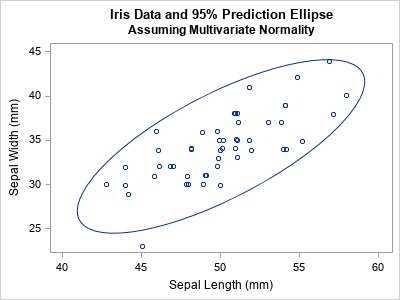
Suppose you have some data that you think are approximately multivariate normal. You can use the log-likelihood function to evaluate whether the model MVN(μ₁, Σ₁) fits the data better than an alternative model MVN(μ₂, Σ₂). For example, the Fisher Iris data for the SepalLength and SepalWidth variables appear to be approximately bivariate normal and positively correlated, as shown in the following graph:

title "Iris Data and 95% Prediction Ellipse";
title2 "Assuming Multivariate Normality";
proc sgplot data=Sashelp.Iris noautolegend;
   where species="Setosa";
   scatter x=SepalLength y=SepalWidth / jitter;
   ellipse x=SepalLength y=SepalWidth;
run;

The following SAS/IML function defines a function (LogPdfMVN) that evaluates the log-PDF at every observation of a data matrix, given the MVN parameters (or estimates for the parameters). To test the function, the program creates a data matrix from the SepalLength and SepalWidth variables for the observations for which Species="Setosa". The program uses the MEAN and COV functions to compute the maximum likelihood estimates for the data, then calls the LogPdfMVN function to evaluate the log-PDF at each observation:

proc iml;
/* This function returns the log-PDF for a MVN(mu, Sigma) density at each row of X.
   The output is a vector with the same number of rows as X. */
start LogPdfMVN(X, mu, Sigma);
   d = ncol(X);
   log2pi = log( 2*constant('pi') );
   logdet = logabsdet(Sigma)[1];             /* sign of det(Sigma) is '+' */
   MDsq = mahalanobis(X, mu, Sigma)##2;      /* (x-mu)`*inv(Sigma)*(x-mu) */
   Y = -0.5 *( MDsq + d*log2pi + logdet );   /* log-PDF for each obs. Sum it for LL */
   return( Y );
finish;
 
/* read the iris data for the Setosa species */
use Sashelp.Iris where(species='Setosa');
read all var {'SepalLength' 'SepalWidth'} into X;
close;
 
n = nrow(X);           /* assume no missing values */
m = mean(X);           /* maximum likelihood estimate of mu */
S = (n-1)/n * cov(X);  /* maximum likelihood estimate of Sigma */
/* evaluate the log likelihood for each observation */
LL = LogPdfMVN(X, m, S);

Notice that you can find the maximum likelihood estimates (m and S) by using a direct computation. For MVN models, you do not need to run a numerical optimization, which is one reason why MVN models are so popular.

The LogPdfMVN function returns a vector that has the same number of rows as the data matrix. The value of the i_th element is the log-PDF of the i_th observation, given the parameters. Because the parameters for the LogPdfMVN function are the maximum likelihood estimates, the total log likelihood (the sum of the LL vector) should be as large as possible for this data. In other words, if we choose different values for μ and Σ, the total log likelihood will be less. Let's see if that is true for this example. Let's change the mean vector and use a covariance matrix that incorrectly postulates that the SepalLength and SepalWidth variables are negatively correlated. The following statements compute the log likelihood for the alternative model:

/* What if we use "wrong" parameters? */
m2 = {45 30};
S2 = {12 -10,  -10 14};          /* this covariance matrix indicates negative correlation */
LL_Wrong = LogPdfMVN(X, m2, S2); /* LL for each obs of the alternative model */
 
/* The total log likelihood is sum(LL) over all obs */
TotalLL = sum(LL);
TotalLL_Wrong = sum(LL_Wrong);
print TotalLL TotalLL_Wrong;

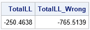
As expected, the total log likelihood is larger for the first model than for the second model. The interpretation that the first model fits the data better than the second model.

Although the total log likelihood (the sum) is often used to choose the better model, the log-PDF of the individual observations are also important. The individual log-PDF values identify which observations are unlikely to come from a distribution with the given parameters.

Visualize the log-likelihood for each model

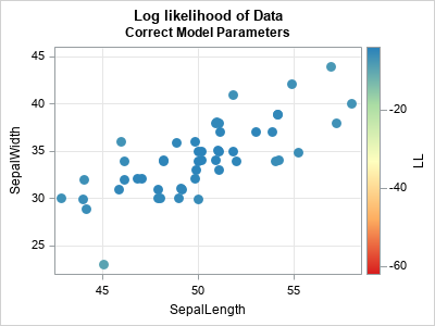
The easiest way to demonstrate the difference between the "good" and "bad" model parameters is to draw the bivariate scatter plot of the data and color each observation by the log-PDF at that position.

The plot for the first model (which fits the data well) is shown below. The observations are colored by the log-PDF value (the LL vector) for each observation. Most observations are blue or blue-green because those colors indicate high values of the log-PDF.

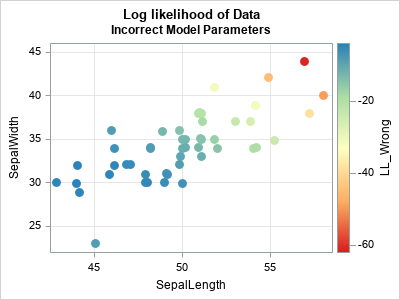
The plot for the second model (which intentionally misspecifies the parameters) is shown below. The observations near (45, 30) are blue or blue-green because that is the location of the specified mean parameter. A prediction ellipse for the specified model has a semimajor axis that slopes from the upper left to the lower right. Therefore, the points in the upper right corner of the plot have a large Mahalanobis distance and a very negative log-PDF. These points are colored yellow, orange, or red. They are "outliers" in the sense that they are unlikely to be observed in a random sample from an MVN distribution that has the second set of parameters.

What is a "large" log-PDF value?

For this example, the log-PDF is negative for each observation, so "large" and "small" can be confusing terms. I want to emphasize two points:

When I say a log-PDF value is "large" or "high," I mean "close to the maximum value of the log-PDF function." For example, -3.1 is a large log-PDF value for these data. Observations that are far from the mean vector are very negative. For example, -40 is a "very negative" value.
The maximum value of the log-PDF occurs when an observation exactly equals the mean vector. Thus the log-PDF will never be larger than -0.5*( d*log(2π) + log(det(Σ)) ). For these data, the maximum value of the log-PDF is -4.01 when you use the maximum likelihood estimates as MVN parameters.

Summary

In summary, this article shows how to evaluate the log-PDF of the multivariate normal distribution. The log-PDF values indicate how likely each observation would be in a random sample, given parameters for an MVN model. If you sum the log-PDF values over all observations, you get a statistic (the total log likelihood) that summarizes how well a model fits the data. If you are comparing two models, the one with the larger log likelihood is the model that fits better.

Blogs