The Kullback–Leibler divergence is a measure of dissimilarity between two probability distributions. An application in machine learning is to measure how distributions in a parametric family differ from a data distribution. This article shows that if you minimize the Kullback–Leibler divergence over a set of parameters, you can find a distribution that is similar to the data distribution. This article focuses on discrete distributions.

The Kullback–Leibler divergence between two discrete distributions

As explained in a previous article, the Kullback–Leibler (K-L) divergence between two discrete probability distributions is the sum
KL(f, g) = Σ_x f(x) log( f(x)/g(x) )
where the sum is over the set of x values for which f(x) > 0. (The set {x | f(x) > 0} is called the support of f.) For this sum to be well defined, the distribution g must be strictly positive on the support of f.

One application of the K-L divergence is to measure the similarity between a hypothetical model distribution defined by g and an empirical distribution defined by f.

Example data for the Kullback–Leibler divergence

As an example, suppose a call center averages about 10 calls per hour. An analyst wants to investigate whether the number of calls per hour can be modeled by using a Poisson(λ=10) distribution. To test the hypothesis, the analyst records the number of calls for each hour during 100 hours of operation. The following SAS DATA step reads the data. The call to PROC SGPLOT creates a histogram shows the distribution of the 100 counts:

data Calls;
input N @@;
label N = "Calls per hour";
datalines;
11 19 11 13 13 8 11 9 9 14 
10 13 8 15 7 9 6 12 7 13 
12 19 6 12 11 12 11 9 15 4 
7 12 12 10 10 16 18 13 13 8 
13 10 9 9 12 13 12 8 13 9 
7 9 10 9 4 10 12 5 4 12 
8 12 14 16 11 7 18 8 10 13 
12 5 11 12 16 9 11 8 11 7 
11 15 8 7 12 16 9 18 9 8 
10 7 11 12 13 15 6 10 10 7 
;
 
title "Number of Calls per Hour";
title2 "Data for 100 Hours";
proc sgplot data=Calls;
   histogram N / scale=proportion binwidth=1;
   xaxis values=(4 to 19) valueshint;
run;

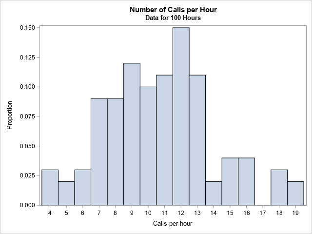
The graph should really be a bar chart, but I used a histogram with BINWIDTH=1 so that the graph reveals that the value 17 does not appear in the data. Furthermore, the values 0, 1, 2, and 3 do not appear in the data. I used the SCALE=PROPORTION option to plot the data distribution on the density scale.

The call center wants to model these data by using a Poisson distribution. The traditional statistical approach is to use maximum likelihood estimation (MLE) to find the parameter, λ, in the Poisson family so that the Poisson(λ) distribution is the best fit to the data. However, let's see how using the Kullback–Leibler divergence leads to a similar result.

The Kullback–Leibler divergence between data and a Poisson distribution

Let's compute the K-L divergence between the empirical frequency distribution and a Poisson(10) distribution. The empirical distribution is the reference distribution; the Poisson(10) distribution is the model. The Poisson distribution has a nonzero probability for all x ≥ 0, but recall that the K-L divergence is computed by summing over the observed values of the empirical distribution, which is the set {4, 5, ..., 19}, excluding the value 17.

proc iml;
/* read the data, which is the reference distribution, f */
use Calls;  read all var "N" into Obs;  close;
call Tabulate(Levels, Freq, Obs);   /* find unique values and frequencies */
Proportion = Freq / nrow(Obs);      /* empirical density of frequency of calls (f) */
 
/* create the model distribution: Poisson(10) */
lambda = 10;   
poisPDF = pdf("Poisson", Levels, lambda); /* Poisson model on support(f) */
 
/* load K-L divergence module or include the definition from: 
 https://blogs.sas.com/content/iml/2020/05/26/kullback-leibler-divergence-discrete.html
*/
load module=KLDiv;
KL = KLDiv(Proportion, poisPDF); 
print KL[format=best5.];

Notice that although the Poisson distribution has infinite support, you only need to evaluate the Poisson density on the (finite) support of empirical density.

Minimize the Kullback–Leibler divergence between data and a Poisson distribution

The previous section shows how to compute the Kullback–Leibler divergence between an empirical density and a Poisson(10) distribution. You can repeat that computation for a whole range of λ values and plot the divergence versus the Poisson parameter. The following statements compute the K-L divergence for λ on [4, 16] and plots the result. The minimum value of the K-L divergence is achieved near λ = 10.7. At that value of λ, the K-L divergence between the data and the Poisson(10.7) distribution is 0.105.

/* Plot the K-L div versus lambda for a sequence of Poisson(lambda) models */
lambda = do(4, 16, 0.1);
KL = j(1, ncol(lambda), .);
do i = 1 to ncol(lambda);
   poisPDF = pdf("Poisson", Levels, lambda[i]);
   KL[i] = KLDiv(Proportion, poisPDF); 
end;
 
title "K-L Divergence from Poisson(lambda)";
call series(lambda, KL) grid={x y} xvalues=4:16 label={'x' 'K-L Divergence'};

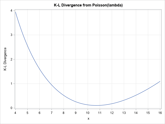
The graph shows the K-L divergence for a sequence of Poisson(λ) models. The Poisson(10.7) model has the smallest divergence from the data distribution, therefore it is the most similar to the data among the Poisson(λ) distributions that were considered. You can use a numerical optimization technique in SAS/IML if you want to find a more accurate value that minimizes the K-L divergences.

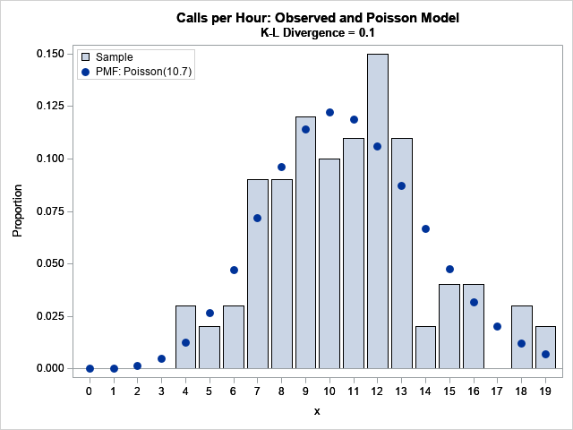
The following graph overlays the PMF for the Poisson(10.7) distribution on the empirical distribution for the number of calls.

The minimal Kullback–Leibler divergence and the maximum likelihood estimate

You might wonder how minimizing the K-L divergence relates to the traditional MLE method for fitting a Poisson model to the data. The following call to PROC GENMOD shows that the MLE estimate is λ = 10.71:

proc genmod data=MyData;
   model Obs = / dist=poisson;
   output out=PoissonFit p=lambda;
run;
 
proc print data=PoissonFit(obs=1) noobs;
   var lambda;
run;

Is this a coincidence? No. It turns out that there a connection between the K-L divergence and the negative log-likelihood. Minimizing the K-L divergence is equivalent to minimizing the negative log-likelihood, which is equivalent to maximizing the likelihood between the Poisson model and the data.

Summary

This article shows how to compute the Kullback–Leibler divergence between an empirical distribution and a Poisson distribution. The empirical distribution was the observed number of calls per hour for 100 hours in a call center. You can compute the K-L divergence for many parameter values (or use numerical optimization) to find the parameter that minimizes the K-L divergence. This parameter value corresponds to the Poisson distribution that is most similar to the data. It turns out that minimizing the K-L divergence is equivalent to maximizing the likelihood function. Although the parameter estimates are the same, the traditional MLE estimate comes with additional tools for statistical inference, such as estimates for confidence intervals and standard errors.

You can also compute the K-L divergence for continuous probability distributions.