The Kullback–Leibler divergence between continuous probability distributions

In a previous article, I discussed the definition of the Kullback-Leibler (K-L) divergence between two discrete probability distributions. For completeness, this article shows how to compute the Kullback-Leibler divergence between two continuous distributions. When f and g are discrete distributions, the K-L divergence is the sum of f(x)*log(f(x)/g(x)) over all x values for which f(x) > 0. When f and g are continuous distributions, the sum becomes an integral:
KL(f,g) = ∫ f(x)*log( f(x)/g(x) ) dx
which is equivalent to
KL(f,g) = ∫ f(x)*( log(f(x)) – log(g(x)) ) dx
The integral is over the support of f, and clearly g must be positive inside the support of f for the integral to be defined.

The Kullback-Leibler divergence between normal distributions

I like to perform numerical integration in SAS by using the QUAD subroutine in the SAS/IML language. You specify the function that you want to integrate (the integrand) and the domain of integration and get back the integral on the domain. Use the special missing value .M to indicate "minus infinity" and the missing value .P to indicate "positive infinity."

As a first example, suppose the f(x) is the pdf of the normal distribution N(μ1, σ1) and g(x) is the pdf of the normal distribution N(μ2, σ2). From the definition, you can exactly calculate the Kullback-Leibler divergence between normal distributions:
KL between Normals: log(σ2/σ1) + (σ1² – σ2² + (μ1 – μ2)²) / (2*σ2²)

You can define the integrand by using the PDF and LOGPDF functions in SAS. The following computation integrates the distributions on the infinite integral (-∞, ∞), although a "six sigma" interval about μ1, such as [-6, 6], would give the same result:

proc iml;
/* Example 1: K-L divergence between two normal distributions */
start KLDivNormal(x) global(mu1, mu2, sigma1, sigma2);
   return pdf("Normal", x, mu1, sigma1) #
          (logpdf("Normal", x, mu1, sigma1) - logpdf("Normal", x, mu2, sigma2));
finish;
 
/* f is PDF for N(0,1) and g is PDF for N(2,3) */ 
mu1 = 0; sigma1 = 1;
mu2 = 2; sigma2 = 3;
 
call quad(KL, "KLDivNormal", {.M .P});  /* integral on (-infinity, infinity) */
KLExact = log(sigma2/sigma1) + 
          (sigma1##2 - sigma2##2+ (mu1-mu2)##2) / (2*sigma2##2);
print KL KLExact (KL-KLExact)[L="Difference"];

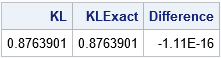
The output indicates that the numerical integration agrees with the exact result to many decimal places.

The Kullback-Leibler divergence between exponential and gamma distributions

A blog post by John D. Cook computes the K-L divergence between an exponential and a gamma(a=2) distribution. This section performs the same computation in SAS.

This is a good time to acknowledge that numerical integration can be challenging. Numerical integration routines have default settings that enable you to integrate a wide variety of functions, but sometimes you need to modify the default parameters to get a satisfactory result—especially for integration on infinite intervals. I have previously written about how to use the PEAK= option for the QUAD routine to achieve convergence in certain cases by providing additional guidance to the QUAD routine about the location and scale of the integrand. Following the advice I gave in the previous article, a value of PEAK=0.1 seems to be a good choice for the K-L divergence between the exponential and gamma(a=2) distributions: it is inside the domain of integration and is close to the mode of the integrand, which is at x=0.

/* Example 2: K-L divergence between exponential and gamma(2). Example from
   https://www.johndcook.com/blog/2017/11/08/why-is-kullback-leibler-divergence-not-a-distance/
*/
start KLDivExpGamma(x) global(a);
   return pdf("Exponential", x) #
          (logpdf("Exponential", x) - logpdf("Gamma", x, a));
finish;
 
a = 2;
/* Use PEAK= option: https://blogs.sas.com/content/iml/2014/08/13/peak-option-in-quad.html */
call quad(KL2, "KLDivExpGamma", {0 .P}) peak=0.1;
print KL2;

The value of the K-L divergence agrees with the answer in John D. Cook's blog post.

Approximating the Exponential Distribution by the Gamma Distribution

Recall that the K-L divergence is a measure of the dissimilarity between two distributions. For example, the previous example indicates how well the gamma(a=2) distribution approximates the exponential distribution. As I showed for discrete distributions, you can use the K-L divergence to select the parameters for a distribution that make it the most similar to another distribution. You can do this by using optimization methods, but I will merely plot the K-L divergence as a function of the shape parameter (a) to indicate how the K-L divergence depends on the parameter.

You might recall that the gamma distribution includes the exponential distribution as a special case. When the shape parameter a=1, the gamma(1) distribution is an exponential distribution. Therefore, the K-L divergence between the exponential and the gamma(1) distribution should be zero.

The following program computes the K-L divergence for values of a in the range [0.5, 2] and plots the K-L divergence versus the parameter:

/* Plot KL(Expo, Gamma(a)) for various values of a.
   Note that gamma(a=1) is the exponential distribution. */
aa = do(0.5, 2, 0.01);
KL = j(1, ncol(aa), .);
do i = 1 to ncol(aa);
   a = aa[i];
   call quad(KL_i, "KLDivExpGamma", {0 .P}) peak=0.1;
   KL[i] = KL_i;
end;
title "Kullback-Leibler Divergence Between Exponential and Gamma{a)";
call series(aa, KL) grid={x y} label={'Gamma Shape Parameter (a)' 'K-L Divergence'};

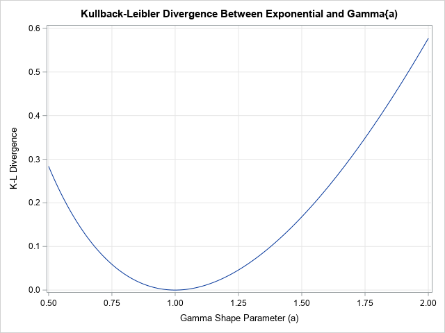
As expected, the graph of the K-L divergence reaches a minimum value at a=1, which is the best approximation to an exponential distribution by the gamma(a) distribution. Note that the K-L divergence equals zero when a=1, which indicates that the distributions are identical when a=1.

Summary

The Kullback-Leibler divergence between two continuous probability distributions is an integral. This article shows how to use the QUAD function in SAS/IML to compute the K-L divergence between two probability distributions.

Blogs