The Kullback–Leibler divergence between discrete probability distributions

If you have been learning about machine learning or mathematical statistics, you might have heard about the Kullback–Leibler divergence. The Kullback–Leibler divergence is a measure of dissimilarity between two probability distributions. It measures how much one distribution differs from a reference distribution. This article explains the Kullback–Leibler divergence and shows how to compute it for discrete probability distributions.

Recall that there are many statistical methods that indicate how much two distributions differ. For example, a maximum likelihood estimate involves finding parameters for a reference distribution that is similar to the data. Statistics such as the Kolmogorov-Smirnov statistic are used in goodness-of-fit tests to compare a data distribution to a reference distribution.

What is the Kullback–Leibler divergence?

Let f and g be probability mass functions that have the same domain. The Kullback–Leibler (K-L) divergence is the sum
KL(f, g) = Σ_x f(x) log( f(x)/g(x) )
where the sum is over the set of x values for which f(x) > 0. (The set {x | f(x) > 0} is called the support of f.) The K-L divergence measures the similarity between the distribution defined by g and the reference distribution defined by f.

For this sum to be well defined, the distribution g must be strictly positive on the support of f. That is, the Kullback–Leibler divergence is defined only when g(x) > 0 for all x in the support of f.

Some researchers prefer the argument to the log function to have f(x) in the denominator. Flipping the ratio introduces a negative sign, so an equivalent formula is
KL(f, g) = –Σ_x f(x) log( g(x)/f(x) )

Notice that if the two density functions (f and g) are the same, then the logarithm of the ratio is 0. Therefore, the K-L divergence is zero when the two distributions are equal. The K-L divergence is positive if the distributions are different.

The Kullback–Leibler divergence was developed as a tool for information theory, but it is frequently used in machine learning. The divergence has several interpretations. In information theory, it measures the information loss when f is approximated by g. In statistics and machine learning, f is often the observed distribution and g is a model.

An example of Kullback–Leibler divergence

As an example, suppose you roll a six-sided die 100 times and record the proportion of 1s, 2s, 3s, etc. You might want to compare this empirical distribution to the uniform distribution, which is the distribution of a fair die for which the probability of each face appearing is 1/6. The following SAS/IML statements compute the Kullback–Leibler (K-L) divergence between the empirical density and the uniform density:

proc iml;
/* K-L divergence is defined for positive discrete densities */
/* Face: 1   2   3   4   5   6 */
f    = {20, 14, 19, 19, 12, 16} / 100;  /* empirical density; 100 rolls of die */
g    = { 1,  1,  1,  1,  1,  1} / 6;    /* uniform density */
KL_fg = -sum( f#log(g/f) );             /* K-L divergence using natural log */
print KL_fg;

The K-L divergence is very small, which indicates that the two distributions are similar.

Although this example compares an empirical distribution to a theoretical distribution, you need to be aware of the limitations of the K-L divergence. The K-L divergence compares two distributions and assumes that the density functions are exact. The K-L divergence does not account for the size of the sample in the previous example. The computation is the same regardless of whether the first density is based on 100 rolls or a million rolls. Thus, the K-L divergence is not a replacement for traditional statistical goodness-of-fit tests.

The Kullback–Leibler is not symmetric

Let's compare a different distribution to the uniform distribution. Let h(x)=9/30 if x=1,2,3 and let h(x)=1/30 if x=4,5,6. The following statements compute the K-L divergence between h and g and between g and h. In the first computation, the step distribution (h) is the reference distribution. In the second computation, the uniform distribution is the reference distribution.

h = { 9,  9,  9,  1,  1,  1} /30;    /* step density */
g = { 1,  1,  1,  1,  1,  1} / 6;    /* uniform density */
KL_hg = -sum( h#log(g/h) );          /* h is reference distribution */
print KL_hg;
 
/* show that K-L div is not symmetric */
KL_gh = -sum( g#log(h/g) );          /* g is reference distribution */
print KL_gh;

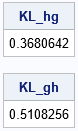
First, notice that the numbers are larger than for the example in the previous section. The f density function is approximately constant, whereas h is not. So the distribution for f is more similar to a uniform distribution than the step distribution is. Second, notice that the K-L divergence is not symmetric. In the first computation (KL_hg), the reference distribution is h, which means that the log terms are weighted by the values of h. The weights from h give a lot of weight to the first three categories (1,2,3) and very little weight to the last three categories (4,5,6). In contrast, g is the reference distribution for the second computation (KL_gh). Because g is the uniform density, the log terms are weighted equally in the second computation.

The fact that the summation is over the support of f means that you can compute the K-L divergence between an empirical distribution (which always has finite support) and a model that has infinite support. However, you cannot use just any distribution for g. Mathematically, f must be absolutely continuous with respect to g. (Another expression is that f is dominated by g.) This means that for every value of x such that f(x)>0, it is also true that g(x)>0.

A SAS function for the Kullback–Leibler divergence

It is convenient to write a function, KLDiv, that computes the Kullback–Leibler divergence for vectors that give the density for two discrete densities. The call KLDiv(f, g) should compute the weighted sum of log( g(x)/f(x) ), where x ranges over elements of the support of f. By default, the function verifies that g > 0 on the support of f and returns a missing value if it isn't. The following SAS/IML function implements the Kullback–Leibler divergence.

/* The Kullback–Leibler divergence between two discrete densities f and g.
   The f distribution is the reference distribution, which means that 
   the sum is probability-weighted by f. 
   If f(x0)>0 at some x0, the model must allow it. You cannot have g(x0)=0.
*/
start KLDiv(f, g, validate=1);
   if validate then do;        /* if g might be zero, validate */
      idx = loc(g<=0);         /* find locations where g = 0 */
      if ncol(idx) > 0 then do; 
         if any(f[idx]>0) then do; /* g is not a good model for f */
            *print "ERROR: g(x)=0 when f(x)>0";
            return( . );
         end;
      end;
   end;
   if any(f<=0) then do;        /* f = 0 somewhere */
      idx = loc(f>0);           /* support of f */
      fp = f[idx];              /* restrict f and g to support of f */
      return -sum( fp#log(g[idx]/fp) );  /* sum over support of f */
   end;
   /* else, f > 0 everywhere */
   return -sum( f#log(g/f) );  /* K-L divergence using natural logarithm */
finish;
 
/* test the KLDiv function */
f = {0, 0.10, 0.40, 0.40, 0.1};
g = {0, 0.60, 0.25, 0.15, 0};
KL_pq = KLDiv(f, g);  /* g is not a valid model for f; K-L div not defined */
KL_qp = KLDiv(g, f);  /* f is valid model for g. Sum is over support of g */
print KL_pq KL_qp;

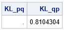
The first call returns a missing value because the sum over the support of f encounters the invalid expression log(0) as the fifth term of the sum. The density g cannot be a model for f because g(5)=0 (no 5s are permitted) whereas f(5)>0 (5s were observed). The second call returns a positive value because the sum over the support of g is valid. In this case, f says that 5s are permitted, but g says that no 5s were observed.

Summary

This article explains the Kullback–Leibler divergence for discrete distributions. A simple example shows that the K-L divergence is not symmetric. This is explained by understanding that the K-L divergence involves a probability-weighted sum where the weights come from the first argument (the reference distribution). Lastly, the article gives an example of implementing the Kullback–Leibler divergence in a matrix-vector language such as SAS/IML. This article focused on discrete distributions. The next article shows how the K-L divergence changes as a function of the parameters in a model. A third article discusses the K-L divergence for continuous distributions.

References

For a mathematical treatment, see "Kullback-Leibler divergence" by Marco Taboga
For an intuitive data-analytic discussion, see "Kullback-Leibler Divergence Explained" by Will Kurt.

Blogs