This is a second article about analyzing longitudinal data, which features measurements that are repeatedly taken on subjects at several points in time. The previous article discusses a response-profile analysis, which uses an ANOVA method to determine differences between the means of an experimental group and a placebo group. The response-profile analysis has limitations, including the fact that longitudinal data are autocorrelated and so do not satisfy the independence assumption of ANOVA. Furthermore, the method does not enable you to model the response profile of individual subjects; it produces only a mean response-by-time profile.

This article shows how a mixed model can produce a response profile for each subject. A mixed model also addresses other limitations of the response-profile analysis. This blog post is based on the introductory article, "A Primer in Longitudinal Data Analysis", by G. Fitzmaurice and C. Ravichandran (2008), Circulation, 118(19), p. 2005-2010.

The data (from Fitzmaurice and C. Ravichandran, 2008) are the blood lead levels for 100 inner-city children who were exposed to lead in their homes. Half were in an experimental group and were given a compound called succimer as treatment. The other half were in a placebo group. Blood-lead levels were measured for each child at baseline (week 0), week 1, week 4, and week 6. The data are visualized in the previous article. You can download the SAS program that creates the data and graphs in this article.

Advantages of the mixed model for longitudinal data

The main advantage of a mixed-effect model is that each subject is assumed to have his or her own mean response curve that explains how the response changes over time. The individual curves are a combination of two parts: "fixed effects," which are common to the population and shared by all subjects, and "random effects," which are specific to each subject. The term "mixed" implies that the model incorporates both fixed and random effects.

You can use a mixed model to do the following:

1. Model the individual response-by-time curves.
2. Model autocorrelation or clusters among observations. This is not discussed further in this blog post.
3. Model time as a continuous variable, which is useful for data that includes mistimed observations and parametric models of time, such as a quadratic model or a piecewise linear model.

The book Applied Longitudinal Analysis (G. Fitzmaurice, N. Laird, and J. Ware, 2011, 2nd Ed.) discusses almost a dozen ways to model the data for blood-lead level in children. This blog post briefly shows how to implement three models in SAS that incorporate random intercepts. The models are the response-profile model, a quadratic model, and a piecewise linear model.

Visualize mixed models

I've previously written about how to visualize mixed models in SAS. One of the techniques is to create a spaghetti plot that shows the predicted response profiles for each subject in the study. Because we will examine three different models, the following statements define a macro that will sort the predicted values and plot them in a spaghetti plot:

%macro SortAndPlot(DSName);
proc sort data=&DSName;
   by descending Treatment ID Time;
run;
 
proc sgplot data=&DSName dattrmap=Order;
   series x=Time y=Pred / group=ID groupLC=Treatment break lineattrs=(pattern=solid)
                       attrid=Treat;
   legenditem type=line name="P" / label="Placebo (P)" lineattrs=GraphData1; 
   legenditem type=line name="A" / label="Succimer (A)" lineattrs=GraphData2; 
   keylegend "A" "P";
   xaxis values=(0 1 4 6) grid;
   yaxis label="Predicted Blood Lead Level (mcg/dL)";
run;
%mend;

A response-profile model with a random intercept

In the response-profile analysis, the data were analyzed by using PROC GLM, although these data do not satisfy the assumptions of PROC GLM. This article uses PROC MIXED in SAS/STAT software for the analyses. You can use the REPEATED statement in PROC MIXED to specify that the measurements for individuals are autocorrelated. We will use an unstructured covariance matrix for the model (TYPE=UN), but Fitzmaurice, Laird, and Ware (2011) discuss other options.

In the response-profile analysis, the model predicts the mean response for each treatment group. However, the baseline measurements for each subject are all different. For example, some start the trial with a blood-lead level that is higher than the mean, others start lower than the mean. To adjust for this variation among subjects, you can use the RANDOM INTERCEPT statement in PROC MIXED. Use the OUTPRED= option on the MODEL statement to write the predicted values for each subject to a data set, then plot the results. The following statements repeat the response-profile model of the previous blog post but include an intercept for each subject.

/* Repeat the response-profile analysis, but 
   use the RANDOM statement to add random intercept for each subject */
proc mixed data=TLCView;
   class id Time(ref='0') Treatment(ref='P');
   model y = Treatment Time Treatment*Time / s chisq outpred=MixedOut;
   repeated Time / type=un subject=id r;   /* measurements are repeated for subjects */
   random intercept / subject=id;          /* each subject gets its own intercept */
run;
 
title "Predicted Individual Growth Curves";
title2 "Random Intercept Model";
%SortAndPlot(MixedOut);

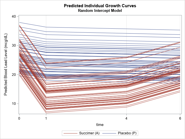
In this model, the shape of the response-profile curve is the same for all subjects in each treatment group. However, the curves are shifted up or down to better match the subject's individual profile.

A mixed model with a quadratic response curve

From the shape of the predicted response curve in the previous section, you might conjecture that a quadratic model might fit the data. You can fit a quadratic model in PROC MIXED by treating Time as a continuous variable. However, Time is also used in the REPEATED statement, and that statement requires a discrete CLASS variable. A resolution to this problem is to create a copy of the Time variable (call it T). You can include T in the CLASS and REPEATED statements and use Time in the MODEL statement as a continuous effect. The third analysis will require a linear spline variable, so the DATA VIEW also creates that variable, called T1.

/* Make "discrete time" (t) to use in REPEATED statement.
   Make spline effect with knot at t=1. */
data TLCView / view=TLCView;
set tlc;
t = Time;                       /* discrete copy of time */
T1 = ifn(Time<1, 0, Time - 1);  /* knot at Time=1 for PWL analysis */
run;

You can now use Time as a continuous effect and T to specify that measurements are repeated for the subjects.

/* Model time as continuous and use a quadratic model in Time. 
   For more about quadratic growth models, see
   https://support.sas.com/resources/papers/proceedings/proceedings/sugi27/p253-27.pdf */
proc mixed data=TLCView;
   class id t(ref='0') Treatment(ref='P');
   model y = Treatment Time Time*Time Treatment*Time / s outpred=MixedOutQuad;
   repeated t / type=un subject=id r;      /* measurements are repeated for subjects */
   random intercept / subject=id;          /* each subject gets its own intercept */
run;
 
title2 "Random Intercept; Quadratic in Time";
%SortAndPlot(MixedOutQuad);

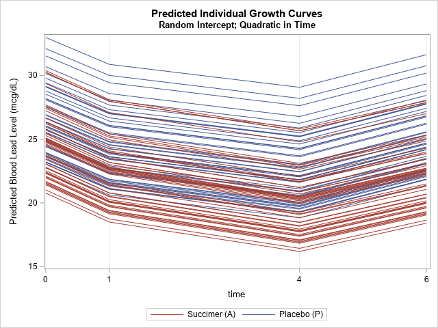
The graph shows the individual predicted responses for each subject, but the quadratic model does not seem to capture the dramatic drop in the blood-lead level at T=1.

A mixed model with a piecewise linear response curve

The next model uses a piecewise linear model instead of a quadratic model. I've previously written about how to use spline effects in SAS to model data by using piecewise polynomials.

For the four time points, the mean response profile seems to go down for the experimental (succimer) group until T=1, and then increase at approximately a constant rate. Is this behavior caused by an underlying biochemical process? I don't know, but if you believe (based on domain knowledge) that this reflects an underlying process, you can incorporate that belief in a piecewise linear model. The first linear segment models the blood-lead level for T ≤ 1; the other segment models the blood-lead level for T > 1.

/* Piecewise linear (PWL) model with knot at Time=1.
   For more about PWL models, see Hwang (2015) 
   "Hands-on Tutorial for Piecewise Linear Mixed-effects Models Using SAS PROC MIXED"
   https://www.lexjansen.com/pharmasug-cn/2015/ST/PharmaSUG-China-2015-ST08.pdf    */
proc mixed data=TLCView;
   class id t(ref='0') Treatment(ref='P');
   model y = Treatment Time T1 Treatment*Time Treatment*T1 / s outpred=MixedOutPWL;
   repeated t / type=un subject=id r;      /* measurements are repeated for subjects */
   random intercept / subject=id;          /* each subject gets its own intercept */
run;
 
title2 "Random Intercept; Piecewise Linear Model";
%SortAndPlot(MixedOutPWL);

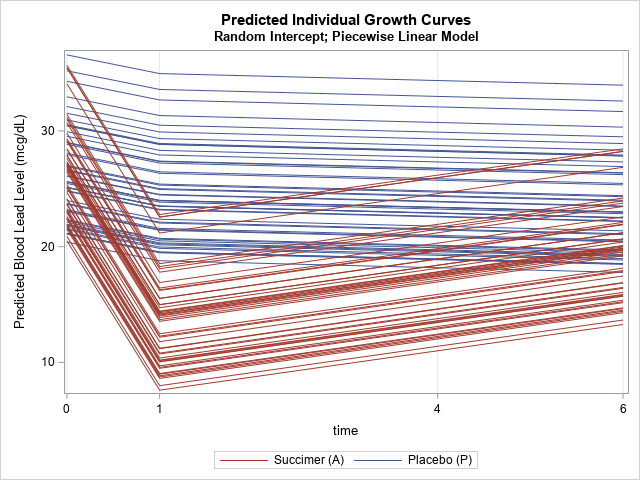
This graph shows a model that is piecewise linear. It assumes that the blood-lead level falls constantly during the first week of the treatment, then either falls or rises constantly during the remainder of the study. You could use the slopes of the lines to report the average rate of change during each time period.

Further reading

There are many papers and many books written about mixed models in SAS. This article presents data and ideas that are discussed in detail in the book Applied Longitudinal Analysis (2012, 2nd Ed) by G. Fitzmaurice, N. Laird, and J. Ware. For an informative article about piecewise-linear mixed models, see Hwang (2015) "Hands-on Tutorial for Piecewise Linear Mixed-effects Models Using SAS PROC MIXED" For a comprehensive discussion of mixed models and repeated-measures analysis, I recommend SAS for Mixed Models, either the 2nd edition or the new edition.

Many people have questions about how to model longitudinal data in SAS. Post your questions to the SAS Support Communities, which has a dedicated community for statistical analysis.