This article shows how to use SAS to fit a growth curve to data. Growth curves model the evolution of a quantity over time. Examples include population growth, the height of a child, and the growth of a tumor cell. This article focuses on using PROC NLIN to estimate the parameters in a nonlinear least squares model. PROC NLIN is my first choice for fitting nonlinear parametric models to data. Other ways to model growth curves include using splines, mixed models (PROC MIXED or NLMIXED), and nonparametric methods such as loess.

The SAS DATA step specifies the mean height (in centimeters) of 58 sunflowers at 7, 14, ..., 84 days after planting. The American naturalist H. S. Reed studied these sunflowers in 1919 and used the mean height values to formulate a model for growth. Unfortunately, I do not have access to the original data for the 58 plants, but using the mean values will demonstrate the main ideas of fitting a growth model to data.

/* Mean heights of 58 sunflowers:
 Reed, H. S. and Holland, R. H. (1919), "Growth of sunflower seeds" 
 Proceedings of the National Academy of Sciences, volume 5, p. 140.
 http://www.pnas.org/content/pnas/5/4/135.full.pdf
*/
data Sunflower;
input Time Height;
label Time = "Time (days)"
      Height="Sunflower Height (cm)";
datalines;
7  17.93
14 36.36
21 67.76
28 98.1
35 131
42 169.5
49 205.5
56 228.3
63 247.1
70 250.5
77 253.8
84 254.5
;

Fit a logistic growth model to data

A simple mathematical model for population growth that is constrained by resources is the logistic growth model, which is also known as the Verhulst growth model. (This should not be confused with logistic regression, which predicts the probability of a binary event.) The Verhulst equation can be parameterized in several ways, but a popular parameterization is
Y(t) = K / (1 + exp(-r*(t – b)))
where

1. K is the theoretical upper limit for the quantity Y. It is called the carrying capacity in population dynamics.
2. r is the rate of maximum growth.
3. b is a time offset. The time t = b is the time at which the quantity is half of its maximum value.

The model has three parameters, K, r, and b. When you use PROC NLIN in SAS to fit a model, you need to specify the parametric form of the model and provide an initial guess for the parameters, as shown below:

 
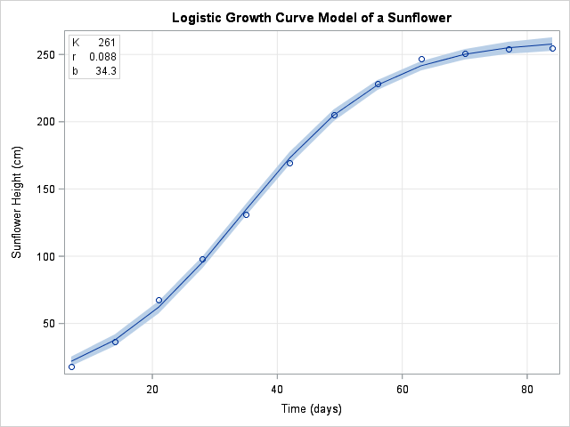
proc nlin data=Sunflower list noitprint;
   parms K 250 r 1 b 40;                         /* initial guess */
   model Height = K / (1 + exp(-r*(Time - b)));  /* model to fit; Height and Time are variables in data */
   output out=ModelOut predicted=Pred lclm=Lower95 uclm=Upper95;
   estimate 'Dt' log(81) / r;                    /* optional: estimate function of parameters */
run;
 
title "Logistic Growth Curve Model of a Sunflower";
proc sgplot data=ModelOut noautolegend;
   band x=Time lower=Lower95 upper=Upper95;         /* confidence band for mean */
   scatter x=Time y=Height;                         /* raw observations */
   series x=Time y=Pred;                            /* fitted model curve */
   inset ('K' = '261'  'r' = '0.088'  'b' = '34.3') / border opaque; /* parameter estimates */
   xaxis grid; yaxis grid;
run;

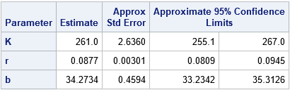
The output from PROC NLIN includes an ANOVA table (not shown), a parameter estimates table (shown below), and an estimate for the correlation of the parameters. The parameter estimates include estimates, standard errors, and 95% confidence intervals for the parameters. The OUTPUT statement creates a SAS data set that contains the original data, the predicted values from the model, and a confidence interval for the predicted mean. The output data is used to create a "fit plot" that shows the model and the original data.

Articles about the Verhulst model often mention that the "maximum growth rate" parameter, r, is sometimes replaced by a parameter that specifies the time required for the population to grow from 10% to 90% of the carrying capacity, K. This time period is called the "characteristic duration" and denoted as Δt. You can show that Δt = log(81)/r. The ESTIMATE statement in PROC NLIN produces a table (shown below) that estimates the characteristic duration.

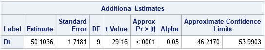
The value 50.1 tells you that, on average, it takes about 50 days for a sunflower to grow from 10 percent of its maximum height to 90 percent of its maximum height. By looking at the graph, you can see that most growth occurs during the 50 days between Day 10 and Day 60.

This use of the ESTIMATE statement can be very useful. Some models have more than one popular parameterization. You can often fit the model for one parameterization and use the ESTIMATE statement to estimate the parameters for a different parameterization.