It is sometimes necessary for researchers to simulate data with thousands of variables. It is easy to simulate thousands of uncorrelated variables, but more difficult to simulate thousands of correlated variables. For that, you can generate a correlation matrix that has special properties, such as a Toeplitz matrix or a first-order autoregressive (AR(1)) correlation matrix. I have previously written about how to generate a large Toeplitz matrix in SAS. This article describes three useful results for an AR(1) correlation matrix:

• How to generate an AR(1) correlation matrix in the SAS/IML language
• How to use a formula to compute the explicit Cholesky root of an AR(1) correlation matrix.
• How to efficiently simulate multivariate normal variables with AR(1) correlation.

Generate an AR(1) correlation matrix in SAS

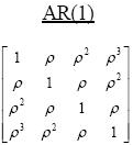
The AR(1) correlation structure is used in statistics to model observations that have correlated errors. (For example, see the documentation of PROC MIXED in SAS.) If Σ is AR(1) correlation matrix, then its elements are constant along diagonals. The (i,j)th element of an AR(1) correlation matrix has the form Σ[i,j] = ρ^{|i – j|}, where ρ is a constant that determines the geometric rate at which correlations decay between successive time intervals. The exponent for each term is the L₁ distance between the row number and the column number. As I have shown in a previous article, you can use the DISTANCE function in SAS/IML 14.3 to quickly evaluate functions that depend on the distance between two sets of points. Consequently, the following SAS/IML function computes the correlation matrix for a p x p AR(1) matrix:

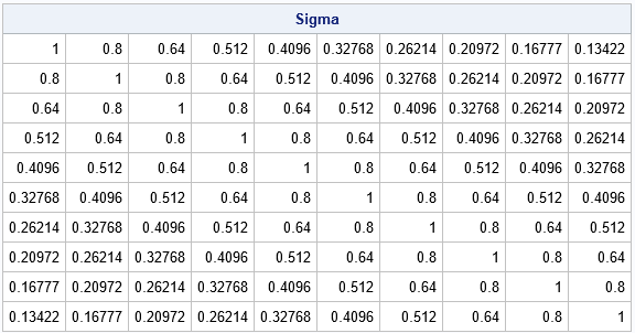
proc iml;
/* return p x p matrix whose (i,j)th element is rho^|i - j| */
start AR1Corr(rho, p); 
   return rho##distance(T(1:p), T(1:p), "L1");
finish;
 
/* test on 10 x 10 matrix with rho = 0.8 */
rho = 0.8;  p = 10;
Sigma = AR1Corr(rho, p);
print Sigma[format=Best7.];

A formula for the Cholesky root of an AR(1) correlation matrix

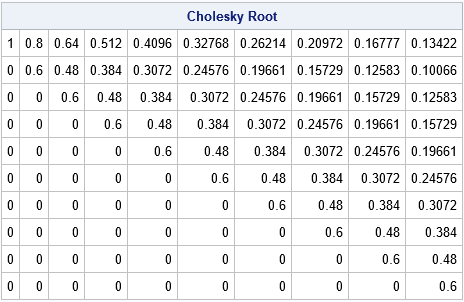
Every covariance matrix has a Cholesky decomposition, which represents the matrix as the crossproduct of a triangular matrix with itself: Σ = R^TR, where R is upper triangular. In SAS/IML, you can use the ROOT function to compute the Cholesky root of an arbitrary positive definite matrix. However, the AR(1) correlation matrix has an explicit formula for the Cholesky root in terms of ρ. This explicit formula does not appear to be well known by statisticians, but it is a special case of a general formula developed by V. Madar (Section 5.1, 2016), who presented a poster at a Southeast SAS Users Group (SESUG) meeting a few years ago. An explicit formula means that you can compute the Cholesky root matrix, R, in a direct and efficient manner, as follows:

/* direct computation of Cholesky root for an AR(1) matrix */
start AR1Root(rho, p);
   R = j(p,p,0);                /* allocate p x p matrix */
   R[1,] = rho##(0:p-1);        /* formula for 1st row */
   c = sqrt(1 - rho**2);        /* scaling factor: c^2 + rho^2 = 1 */
   R2 = c * R[1,];              /* formula for 2nd row */
   do j = 2 to p;               /* shift elements in 2nd row for remaining rows */
      R[j, j:p] = R2[,1:p-j+1]; 
   end;
   return R;
finish;
 
R = AR1Root(rho, p);   /* compare to R = root(Sigma), which requires forming Sigma */
print R[L="Cholesky Root" format=Best7.];

You can compute an AR(1) covariance matrix from the correlation matrix by multiplying the correlation matrix by a positive scalar, σ².

Efficient simulation of multivariate normal variables with AR(1) correlation

An efficient way to simulate data from a multivariate normal population with covariance Σ is to use the Cholesky decomposition to induce correlation among a set of uncorrelated normal variates. This is the technique used by the RandNormal function in SAS/IML software. Internally, the RandNormal function calls the ROOT function, which can compute the Cholesky root of an arbitrary positive definite matrix.

When there are thousands of variables, the Cholesky decomposition might take a second or more. If you call the RandNormal function thousands of times during a simulation study, you pay that one-second penalty during each call. For the AR(1) covariance structure, you can use the explicit formula for the Cholesky root to save a considerable amount of time. You also do not need to explicitly form the p x p matrix, Σ, which saves RAM. The following SAS/IML function is an efficient way to simulate N observations from a p-dimensional multivariate normal distribution that has an AR(1) correlation structure with parameter ρ:

/* simulate multivariate normal data from a population with AR(1) correlation */
start RandNormalAR1( N, Mean, rho );
    mMean = rowvec(Mean);
    p = ncol(mMean);
    U = AR1Root(rho, p);      /* use explicit formula instead of ROOT(Sigma) */
    Z = j(N,p);
    call randgen(Z,'NORMAL');
    return (mMean + Z*U);
finish;
 
call randseed(12345);
p = 1000;                  /* big matrix */
mean = j(1, p, 0);         /* mean of MVN distribution */
 
/* simulate data from MVN distribs with different values of rho */
v = do(0.01, 0.99, 0.01);  /* choose rho from list 0.01, 0.02, ..., 0.99 */
t0 = time();               /* time it! */
do i = 1 to ncol(v);
   rho = v[i];
   X = randnormalAR1(500, mean, rho);  /* simulate 500 obs from MVN with p vars */
end;
t_SimMVN = time() - t0;     /* total time to simulate all data */
print t_SimMVN;

The previous loop generates a sample that contains N=500 observations and p=1000 variables. Each sample is from a multivariate normal distribution that has an AR(1) correlation, but each sample is generated for a different value of ρ, where ρ = 0.01. 0.02, ..., 0.99. On my desktop computer, this simulation of 100 correlated samples takes about 4 seconds. This is about 25% of the time for the same simulation that explicitly forms the AR(1) correlation matrix and calls RandNormal.

In summary, the AR(1) correlation matrix is an easy way to generate a symmetric positive definite matrix. You can use the DISTANCE function in SAS/IML 14.3 to create such a matrix, but for some applications you might only require the Cholesky root of the matrix. The AR(1) correlation matrix has an explicit Cholesky root that you can use to speed up simulation studies such as generating samples from a multivariate normal distribution that has an AR(1) correlation.