You can use the Cholesky decomposition of a covariance matrix to simulate data from a correlated multivariate normal distribution. This method is encapsulated in the RANDNORMAL function in SAS/IML software, but you can also perform the computations manually by calling the ROOT function to get the Cholesky root and then use matrix multiplication to correlate multivariate norm (MVN) data, as follows:
%let d = 12; /* number of variables */ %let N = 500; /* number of observations */ proc iml; d = &d; /* want to generate d variables that are MVN */ N = &N; /* sample size */ /* easy to generate uncorrelated MVN variables */ call randseed(1234); z = j(d, N); call randgen(z, "Normal"); /* z is MVN(0,I(d)) */ /* use Cholesky root to transform to correlated variables */ Sigma = toeplitz(d:1); /* example of covariance matrix */ G = root(Sigma); /* the Cholesky root of the full covariance matrix */ x = G`*z; /* x is MVN(0, Sigma) */ title "Two Components of MVN(0,Sigma) Data"; call scatter(x[1,], x[2,]) label={x1 x2}; |
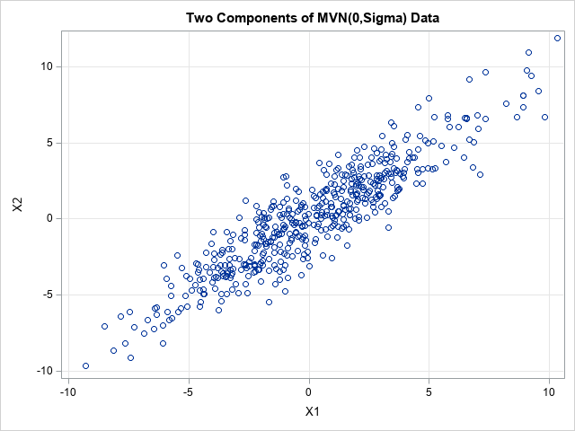
The simulation creates d=12 correlated variables and 500 observations. The first two variables are plotted against each other so that you can see that they are correlated. The other pairs of variables are also correlated according to the entries in the Σ covariance matrix.
Generating a huge number of MVN variables
In the comments to one of my previous articles, a SAS programmer asked whether it is possible to generate MVN data even if the covariance matrix is so large that it cannot be factored by the ROOT function. For example, suppose you want to generate d=20,000 MVN variables. A d x d covariance matrix of that size requires 3 GB of RAM, and on some operating system you cannot form the Cholesky root of a matrix that large. However, I have developed an algorithm that enables you to deal with the covariance matrix (Σ) as a block matrix.
To introduce the algorithm, represent the Σ matrix as a 2 x 2 block matrix. (See the last section for a more general representation.) For a 2 x 2 block algorithm, you only need to form the Cholesky roots of matrices of size (d/2), which are 10000 x 10000 matrices for this example. Matrices of that size require only 0.75 GB and can be quickly factored. Of course, there is no such thing as a free lunch: The new algorithm is more complicated and requires additional computations, albeit on smaller matrices.
Let's look at how to simulate MVN data by treating Σ as a block matrix of size d/2. For ease of exposition, assume d is even and each block is of size d/2. However, the algorithm easily handles the case where d is odd. When d is odd, choose the upper blocks to have floor(d/2) rows and choose the lower clocks to have ceil(d/2) rows. The SAS code (below) handles the general case. (In fact, the algorithm doesn't care about the block size. For any p in (0, 1), one block can be size pd and the other size (1-p)d.
In block form, the covariance matrix is
\(\Sigma = \begin{bmatrix}A & B\\B^\prime & C\end{bmatrix}\)
There is a matrix decomposition called the LDLT decomposition that enables you to write Σ as the product of three block matrices:
\(\begin{bmatrix}A & B\\B^\prime & C\end{bmatrix} =
\begin{bmatrix}I & 0\\B^\prime A^{-1} & I\end{bmatrix}
\begin{bmatrix}A & 0\\0 & S\end{bmatrix}
\begin{bmatrix}I & A^{-1}B\\0 & I\end{bmatrix}
\)
where \(S = C - B^\prime A^{-1} B\) is the Schur complement of the block matrix C.
There is a theorem that says that if Σ is symmetric positive definite (SPD), then so is every principal submatrix, so A is SPD. Thus, we can use the Cholesky decomposition and write \(A = G^\prime_A G_A\) for an upper triangular matrix, \(G_A\). By reordering the variables, C is SPD as well. You can also prove (see Prop 2.2 in these notes by Jean Gallier) that Σ and A are PD if and only if S is PD. Thus you can factor \(S = G^\prime_S G_S\) for an upper triangular Cholesky matrix \(G_S\). (Thanks to my colleague, Clay, for finding this result for me.)
Using these definitions, the Cholesky decomposition of Σ can be written in block form as
\(\Sigma =
\begin{bmatrix}G^\prime_A & 0\\B^\prime G^{-1}_A & G^\prime_S\end{bmatrix}
\begin{bmatrix}G_A & (G^\prime_A)^{-1} B \\ 0 & G_S\end{bmatrix}
\)
To simulate MVN data, we let z be uncorrelated MVN(0, I) data and define
\(x =
\begin{bmatrix}x_1 \\ x_2 \end{bmatrix} =
\begin{bmatrix}G^\prime_A & 0\\B^\prime G^{-1}_A & G^\prime_S\end{bmatrix}
\begin{bmatrix}z_1 \\ z_2\end{bmatrix} =
\begin{bmatrix}G^\prime_A z_1 \\ B^\prime G^{-1}_A z_1 + G^\prime_S z_2\end{bmatrix}
\)
The previous equation indicates that you can generate correlated MVN(0, Σ) data if you know the Cholesky decomposition of the upper-left block of Σ (which is GA) and the Cholesky decomposition of the Schur complement (which is GS). Each of the matrices in these equations is of size d/2, which means that the computations are performed on matrices that are half the size of Σ. However, notice that generating the x2 components requires some extra work: the Schur complement involves the inverse of A and the formula for x2 also involves the inverse of GA. These issues are not insurmountable, but it means that the block algorithm is more complicated than the original algorithm, which merely multiplies z by the Cholesky root of Σ.
A SAS program for block simulation of MVN data
The SAS/IML program in a previous section shows how to generate correlated MVN(0, Σ) data (x) from uncorrelated MVN(0, I) data (z) by using the Cholesky root (G) of Σ. This section shows how to get exactly the same x values by performing block operations. For the block operations, each matrix is size d/2, so has 1/4 of the elements of Σ.
The first step is to represent Σ and z in block form.
/* The Main Idea: get the same MVN data by performing block operations on matrices that are size d/2 */ /* 1. Represent Sigma={A B, B` C} and z={z1, z2} in block form */ d1 = ceil(d/2); /* half the variables */ d2 = d - d1; /* the other half of the vars */ dp1 = d1 + 1; A = Sigma[1:d1, 1:d1]; /* break up the symmetric (d x d) covariance */ B = Sigma[1:d1, dp1:d]; /* matrix into blocks of size d/2 */ C = Sigma[dp1:d, dp1:d]; z1 = z[1:d1, ]; /* extract the first d1 obs for MVN(0,I) data */ z2 = z[dp1:d, ]; /* extract the last d2 obs for MVN(0,I) data */ |
It is easy to generate x1, which contains the first d/2 components of the MVN(0, Σ) simulated data. You simply use the Cholesky decomposition of A, which is the upper-left block of Σ:
/* 2. Compute Cholesky root of A and compute x1 z1 */ G_A = root(A); /* Cholesky of upper left block */ x1 = G_A`*z1; /* generate first half of variables */ |
It is not as easy to generate x2, which contains the last d/2 components. In block form, \(x_2 = v + u\), where \(v = B^\prime G_A^{-1} z_1\) and \(u = G_S^\prime z_2\), and where \(S = G_S^\prime G_S\) is the Cholesky decomposition of the Shur complement. This is shown in the following statements:
/* 3. Generate the second half of variables */ S = C - B`*inv(A)*B; /* S is the Schur complement */ G_S = root(S); /* Cholesky root of Schur complement */ v = B`*inv(G_A)*z1; u = G_S`*z2; x2 = v + u; /* verify that the computation gives exactly the same simulated data */ print (max(abs(x[1:d1,] - x1)))[L="Diff(x - x1)"]; print (max(abs(x[dp1:d,] - x2)))[L="Diff(x - x2)"]; |
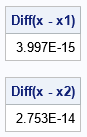
The output shows that the block computation, which uses multiple matrices of size d/2, gives exactly the same answer as the original computation, which uses matrices of size d.
Analysis of the block algorithm
Now that the algorithm runs on a small example, you can increase the dimensions of the matrices. For example, try rerunning the algorithm with the following parameters:
%let d = 5000; /* number of variables */ %let N = 1000; /* number of observations */ |
When I run this larger program on my PC, it takes about 2.3 seconds to simulate the MVN data by using the full Cholesky decomposition. It takes about 17 seconds to simulate the data by using the block method. Most of the time for the block method is spent on the computation v = B`*inv(G_A)*z1, which takes about 15 seconds. So if you want to improve the performance, you should focus on improving that computation.
You can improve the performance of the block algorithm in several ways:- You don't need to find the inverse of A. You have the Cholesky root of A, which is triangular, so you can define H = inv(G`A)*B and compute the Schur complement as C – H`*H.
- You don't need to explicitly form any inverses. Ultimately, all these matrices are going to operate on the vector z2, which means that you can simulate the data by using only matrix multiplication and solving linear equations.
I tried several techniques, but I could not make the block algorithm competitive with the performance of the original Cholesky algorithm. The issue is that the block algorithm computes two Cholesky decompositions, solves some linear equations, and performs matrix multiplication. Even though each computation is on a matrix that is half the size of the original matrix, the additional computations result in a longer runtime.
Generalization to additional blocks
The algorithm generalizes to other block sizes. I will outline the case for a 3 x 3 block matrix. The general case of k x k blocks follows by induction.
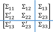
The figure to the right shows the Σ covariance matrix as a 3 x 3 block matrix. By using 2 x 2 block algorithm, you can obtain multivariate normal vectors x1 and x2, which correspond to the covariances in the four blocks in the upper-left corner of the matrix. You can then view the upper four blocks as a single (larger) block, thus obtaining a 2 x 2 block matrix where the upper-left block has size 2d/3 and the lower-right block (Σ33) has size d/3.
There are many details to work through, but the main idea is that you can repeat the computation on this new block matrix where the block sizes are unequal. To proceed, you need the Cholesky decomposition of the large upper-left block, but we have already shown how to compute that in terms of the Cholesky root of Σ11, its inverse, and the Cholesky root of the Schur complement of Σ22. You also need to form the Schur complement of Σ33, but that is feasible because we have the Cholesky decomposition of the large upper-left block.
I have not implemented the details because it is not clear to me whether three or more blocks provides a practical advantage. Even if I work out the details for k=3, the algebra for k > 3 blocks seems to be daunting.
Summary
It is well known that you can use the Cholesky decomposition of a covariance matrix to simulate data from a correlated multivariate normal distribution. This article shows how to break up the task by using a block Cholesky method. The method is implemented for k=2 blocks. The block method requires more matrix operations, but each operation is performed on a smaller matrix. Although the block method takes longer to run, it can be used to generate a large number of variables by generating k variables at a time, where k is small enough that the k x k matrices can be easily handled.
The block method generalizes to k > 2 blocks, but it is not clear whether more blocks provide any practical benefits.

2 Comments
Hi Rick,
I came across this algorithm while trying to come up with a way to save time evaluating a block matrix I'm dealing with. This is really helpful! I was wondering if you knew of a source such as a standard textbook which gives the Cholesky decomposition result you showed. I'd like to have something to cite rather than work out all the math in my application.
Thanks,
Spencer
> I was wondering if you knew of a source such as a standard textbook which gives the Cholesky decomposition result you showed
I'm not sure which "result" you are referring to. If you are referring to the matrix equation after the phrase "the Cholesky decomposition of $\Sigma$ can be written in block form as", that identity is true by inspection. Just multiply the factors to obtain the block for of \Sigma. If you are referring to the L*D*L` decomposition, you can refer to Golub and Van Loan "Matrix Computations" (2nd Ed), p. 137-138.