A radial basis function is a scalar function that depends on the distance to some point, called the center point, c. One popular radial basis function is the Gaussian kernel φ(x; c) = exp(-||x – c||² / (2 σ²)), which uses the squared distance from a vector x to the center c to assign a weight. The weighted sum of Gaussian kernels, Σ w_i φ(x; c) arises in many applications in statistics, including kernel density estimation, kernel smoothing, and machine learning algorithms such as support vector machines. It is therefore important to be able to efficiently evaluate a radial basis function and compute a weighted sum of several such kernel functions.

One of the many useful features of the SAS/IML language is its ability to compactly represent matrix and vector expressions. The expression ||x – c|| looks like the distance between two vectors, but in the SAS/IML language the DISTANCE function can handle multiple sets of vectors:

• The DISTANCE function can compute the distance between two vectors of arbitrary dimensions. Thus when x and c are both d-dimensional row vectors, you can compute the distance by using r = DISTANCE(x, c). The result is a scalar distance.
• The DISTANCE function can compute the distance between multiple points and a center. Thus when x is an m x d matrix that contains m points, you can compute the m distances between the points and c by using r = DISTANCE(x, c). Again, the syntax is the same, but now r is an m x 1 vector of distances.
• The DISTANCE function in SAS/IML 14.3 can compute the distance between multiple points and multiple centers. Thus when x is an m x d matrix that contains m points and c is a p x d matrix that contains p centers, you can compute the m*p distances between the points and c by using r = DISTANCE(x, c). The syntax is the same, but now r is an m x p matrix of distances.

A SAS/IML function that evaluates a Gaussian kernel function

The following SAS/IML statements define a Gaussian kernel function. Notice that the function is very compact! To test the function, define one center at C = (2.3, 3.2). Because SAS/IML is a matrix language, you can evaluate the Gaussian kernel on a grid of integer coordinates (x,y) where x is an integer in the range [1,5] and y is in the range [1,8]. Let Z be the matrix of the 40 ordered pairs. The following call evaluates the Gaussian kernel at the grid of points:

proc iml;
/* Radial basis function (Gaussian kernel). If z is m x d and c is n x d, this function
   returns the mxn matrix of values exp( -||z[i,] - c[j,]||**2 / (2*sigma**2) ) */
start GaussKernel(z, c, sigma=1);
   return exp( -distance(z,c)##2 / (2*sigma**2) );
finish;
 
/* test on small data: Z is an 5 x 8 grid and C = {2.3 3.2} */
xPts = 1:5; yPts = 1:8;
Z = expandgrid(xPts, yPts);              /* expand into (8*5) x 2 matrix */
C = {2.3 3.2};                           /* the center */ 
phi = GaussKernel(Z, C);                 /* phi is 40 x 1 vector */
 
print Z phi;                             /* print in expanded form */
phi_Grid = shapecol(phi, ncol(yPts));    /* reshape into grid (optional) */
print phi_Grid[c=(char(xPts)) r=(char(yPts)) F=4.2];

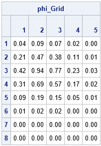
The table shows the Gaussian kernel evaluated at the grid points. The columns represent the values at the X locations and the rows indicate the Y locations. The function is largest at the value (x,y)=(2,3) because (2,3) is the grid point closest to the center (2.3, 3.2). The largest value 0.94. Notice that the function is essentially zero at points that are more than 3 units from the center, which you would expect from a Gaussian distribution with σ = 1.

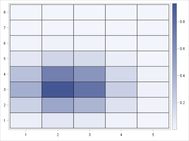
You can use the HEATMAPCONT subroutine to make a heat map of the function values. However, notice that in the matrix the rows increase in the downward direction, whereas in the usual Cartesian coordinate system the Y direction increases upward. Consequently, you need to reverse the rows and the Y-axis labels when you create a heat map:

start PlotValues( v, xPts, yPts );
   G = shapecol(v, ncol(yPts));      /* reshape vector into grid */
   M =  G[nrow(G):1, ];              /* flip Y axis (rows) */
   yRev = yPts[, ncol(yPts):1];      /* reverse the Y-axis labels */
   call heatmapcont(M) xvalues=xPts yValues=yRev;
finish;
run PlotValues(phi, xPts, yPts);

Sums of radial basis functions

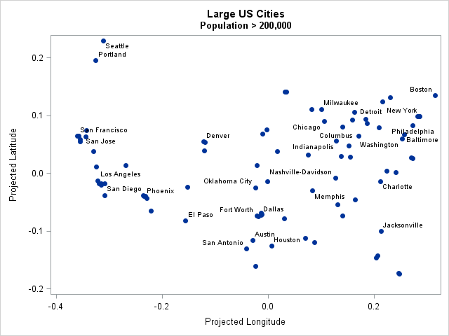
Often the "centers" are the locations of some resource such as a warehouse, a hospital, or an ATM. Let's use the locations of 86 large US cities, which I used in a previous article about spatial data analysis. A graph of the locations of the cities is shown to the right. (Click to enlarge.) The locations are in a standardized coordinate system, so they do not directly correspond to longitudes and latitudes.

If there are multiple centers, the GaussKernel function returns a column for every center. Many applications require a weighted sum of the columns. You can achieve a weighted sum by using a matrix-vector product A*w, where w is a column vector of weights. If you want an unweighted sum, you can use the SAS/IML subscript reduction operator to sum across the columns: A[,+].

For example, the following statements evaluate the Gaussian kernel function at each value in a grid (the Z matrix) and for each of 86 cities (the C matrix). The result is a 3726 x 86 matrix of values. You can use the subscript reduction operator to sum the kernel evaluations over the cities, as shown:

use BigCities;
   read all var {x y} into C;     /* C = (x,y) locations of centers */
   read all var "City";
close;
 
/* Z = a regular grid in (x,y) coordinates that contains the data */
XGridPts = round( do(-0.4, 0.4, 0.01), 0.001);
YGridPts = round( do(-0.2, 0.25, 0.01), 0.001);
Z = expandgrid( XGridPts, YGridPts );  /* 3,726 points on a 81x46 grid */
 
phi = GaussKernel(Z, C, 0.025);   /* use smaller bandwidth */
sumPhi = phi[,+];                 /* for each grid point, add sum of kernel evaluations */

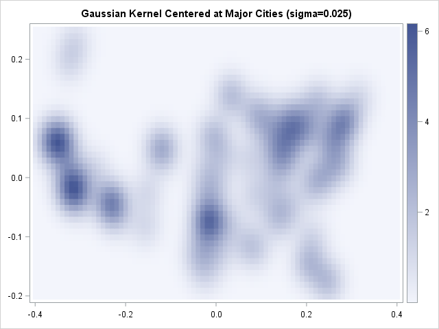
The resulting heat map shows blobs centered at each large city in the data. Locations near isolated cities (such as Oklahoma City) are lighter in color than locations near multiple nearby cities (such as southern California and the New York area) because the image shows the superposition of the kernel functions. At points that are far from any large city, the sum of the Gaussian kernel functions is essentially zero.

In summary, if you work with algorithms that use radial basis functions such as Gaussian kernels, you can use the SAS/IML language to evaluate these functions. By using the matrix features of the language and the fact that the DISTANCE function supports matrices as arguments, you can quickly and efficiently evaluate weighted sums of these kernel functions.