How far away is the nearest hospital? How far is the nearest restaurant? The nearest gas station? These are commonly asked questions whose answers depend on the location of the person asking the question.

Recently I showed an algorithm that enables you to find the distance between a set of locations and a fixed set of reference sites. The set of locations (the people) can be arbitrary, so a good way to summarize the problem is to draw a contour plot that shows the distance from every point in a region to the nearest reference site (a hospital or store). In SAS, you can create this graph by using the SPP procedure, which analyzes spatial point processes. The graph is called an empty-space plot.

Example: The location of large US cities

Some people love big cities and the diverse opportunities that they provide. They want to know how far it is to the nearest big city. Other people hate the noise and congestion; they want to be as far away from a big city as possible. To demonstrate how to create an empty-space plot, let's look at the spatial distribution of US cities that have population more than 200,000.

data BigCities;
set maps.uscity;                          /* part of SAS/GRAPH */
where statecode not in ("AK" "HI" "PR") & pop > 200000;
if pop>500000 then Name=City;             /* label really big cities */
else Name = "        ";
run;
 
title  "Large US Cities";
title2 "Population > 200,000";
proc sgplot data=BigCities;
  scatter x=x y=y / markerattrs=(symbol=CircleFilled) datalabel=Name;
run;

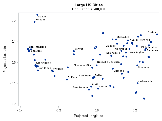
The scatter plot supports a well-known fact: cities are not settled in random locations. People tend to settle near beneficial geographic features, such as proximity to rivers, harbors, and other strategic resources. Therefore the cities are not spread uniformly throughout the country. There are clusters of cities on both coasts and there is a large empty space in the rugged northwest. The large empty space contain locations that are much farther away from a big city than would be expected for a random uniform assortment of 86 cities.

The following call to PROC SPP create an empty-space plot, which reveals regions that are far from a big city. The F option will be explained in a moment:

proc spp data=BigCities plots(equate)=(emptyspace(obs=on) F);
   process BigCities = (x, y / area=(-0.37,-0.19,0.32, 0.24)) / F;
run;

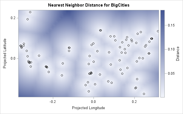
The dark blue color indicates geographic coordinates that are far from any large city. The darkest blue appears to be in the northwestern states, such as Montana, Idaho, and Wyoming. Western Texas also stands out. Those are great places to live for people who want to be far from large cities. There is also dark blue in regions that are uninhabitable (oceans and the Great Lake) or are not part of the US (Mexico and Canada).

I think the image is beautiful, but it is useful as well. It gives a visual summary of locations that are far from the reference sites (big cities).

Empty-space distances

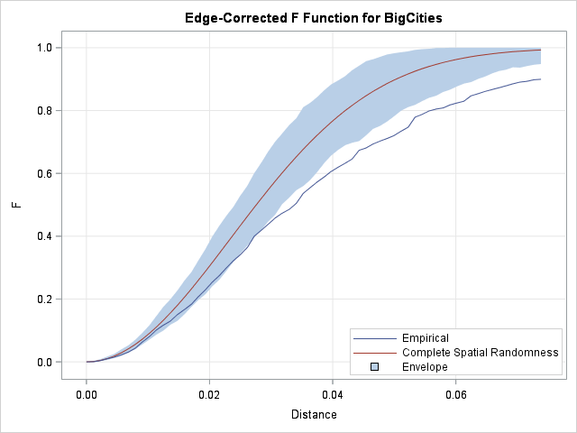
If you want a more statistical analysis, the F option in the PROCESS statement and in the PLOTS= option tells PROC SPP to lay down a regular grid of points and compute the distance from each grid position to the nearest big city. (By default the grid is 50 x 50.) The graph shows the cumulative distribution of these distances in blue. You can compare the distribution of these distances to the expected distribution for randomly selected locations, which is shown in red and labeled "complete spatial randomness."

You can see that the empirical distribution rises more slowly than the theoretical curve. This indicates that the observed locations are more clustered than you would expect if the cities were randomly located. For details about the F option, see the documentation for PROC SPP.

The main purpose of this example is to demonstrate that PROC SPP makes it easy to compute the empty-space plot, which summarizes the distance between an arbitrary location and a pattern of points. In this article the points were large US cities, but obviously you could analyze other point patterns. The SPP procedure has many options that indicate whether the pattern appear to be randomly distributed or clustered. The procedure indicates that the locations of large US cities are not random.