A logistic regression model is a way to predict the probability of a binary response based on values of explanatory variables. It is important to be able to assess the accuracy of a predictive model. This article shows how to construct a calibration plot in SAS. A calibration plot is a goodness-of-fit diagnostic graph. It enables you to qualitatively compare a model's predicted probability of an event to the empirical probability.

Calibration curves

There are two standard ways to assess the accuracy of a predictive model for a binary response: discrimination and calibration. To assess discrimination, you can use the ROC curve. Discrimination involves counting the number of true positives, false positive, true negatives, and false negatives at various threshold values. In contrast, calibration curves compare the predicted probability of the response to the empirical probability. Calibration can help diagnose lack of fit. It also helps to rank subjects according to risk.

This article discusses internal calibration, which is the agreement on the sample used to fit the model. External calibration, which involves comparing the predicted and observed probabilities on a sample that was not used to fit the model, is not discussed.

In the literature, there are two types of calibration plots. One uses a smooth curve to compare the predicted and empirical probabilities. The curve is usually a loess curve, but sometimes a linear regression curve is used. The other (to be discussed in a future article) splits the data into deciles. An extensive simulation study by Austin and Steyerberg (2013) concluded that loess-based calibration curves have several advantages. This article discusses how to use a loess fit to construct a calibration curve.

A calibration curve for a misspecified model

Calibration curves help to diagnose lack of fit. This example simulates data according to a quadratic model but create a linear fit to that data. The calibration curve should indicate that the model is misspecified.

Step 1: Simulate data for a quadratic logistic regression model

Austin and Steyerberg (2013) use the following simulated data, which is based on the earlier work of Hosmer et al. (1997). Simulate X ~ U(-3, 3) and define η = b0 + b1*X + b2*X²) to be a linear predictor, where b0 = -2.337, b1 = 0.8569, b2 = 0.3011. The logistic model is logit(p) = η, where p = Pr(Y=1 | x) is the probability of the binary event Y=1. The following SAS DATA step simulates N=500 observations from this logistic regression model:

/* simulate sample of size N=500 that follows a quadratic model from Hosmer et al. (1997) */
%let N = 500;                              /* sample size */ 
data LogiSim(keep=Y x);
call streaminit(1234);                     /* set the random number seed */
do i = 1 to &N;                            /* for each observation in the sample */
   /* Hosmer et al. chose x ~ U(-3,3). Use rand("Uniform",-3,3) for modern versions of SAS */
   x = -3 + 6*rand("Uniform");
   eta = -2.337 + 0.8569*x + 0.3011*x**2;  /* quadratic model used by Hosmer et al. */
   mu = logistic(eta);
   Y = rand("Bernoulli", mu);
   output;
end;
run;

For this simulated data, the "true" model is known to be quadratic. Of course, in practice, the true underlying model is unknown.

Step 2: Fit a logistic model

The next step is to fit a logistic regression model and save the predicted probabilities. The following call to PROC LOGISTIC intentionally fits a linear model. The calibration plot will indicate that the model is misspecified.

/* Use PROC LOGISTIC and output the predicted probabilities.
   Intentionally MISSPECIFY the model as linear. */
proc logistic data=LogiSim plots=effect;
   model Y(event='1') = x;
   output out=LogiOut predicted=PredProb; /* save predicted probabilities in data set */
run;

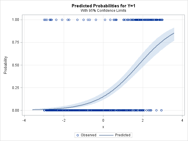
As shown above, PROC LOGISTIC can automatically create a fit plot for a regression that involves one continuous variable. The fit plot shows the observed responses, which are plotted at Y=0 (failure) or Y=1 (success). The predicted probabilities are shown as a sigmoidal curve. The predicted probabilities are in the range (0, 0.8). The next section creates a calibration plot, which is a graph of the predicted probability versus the observed response.

Create the calibration plot

The output from PROC LOGISTIC includes the predicted probabilities and the observed responses. Copas (1983), Harrell et al. (1984), and others have suggested assessing calibration by plotting a scatter plot smoother and overlaying a diagonal line that represents the line of perfect calibration. If the smoother lies close to the diagonal, the model is well calibrated. If there is a systematic deviation from the diagonal line, that indicates that the model might be misspecified.

The following statements sort the data by the predicted probabilities and create the calibration plot. (The sort is optional for the loess smoother, but is useful for other analyses.)

proc sort data=LogiOut;  by PredProb;  run;
 
/* let the data choose the smoothing parameter */
title "Calibration Plot for Misspecified Model";
title2 "True Model Is Quadratic; Fit Is Linear";
proc sgplot data=LogiOut noautolegend aspect=1;
   loess x=PredProb y=y / interpolation=cubic clm;   /* smoothing value by AICC (0.657) */
   lineparm x=0 y=0 slope=1 / lineattrs=(color=grey pattern=dash);
run;

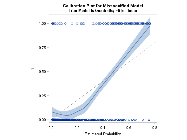
The loess smoother does not lie close to the diagonal line, which indicates that the linear model is not a good fit for the quadratic data. The loess curve is systematically above the diagonal line for very small and very large values of the predicted probability. This indicates that the empirical probability (the proportion of events) is higher than predicted on these intervals. In contrast, when the predicted probability is in the range [0.1, 0.45], the empirical probability is lower than predicted.

Several variations of the calibration plot are possible:

• Add the NOMARKERS option to the LOESS statement to suppress the observed responses.
• Omit the CLM option if you do not want to see a confidence band.
• Use the SMOOTH=0.75 option if you want to specify the value for the loess smoothing parameter. The value 0.75 is the value that Austin and Steyerberg used in their simulation study, in part because that is the default parameter value in the R programming language.
• Use a REG statement instead of the LOESS statement if you want a polynomial smoother.

A calibration plot for a correctly specified model

In the previous section, the model was intentionally misspecified. The calibration curve for the example did not lie close to the diagonal "perfect calibration" line, which indicates a lack of fit. Let's see how the calibration curve looks for the same data if you include a quadratic term in the model. First, generate the predicted probabilities for the quadratic model, then create the calibration curve for the model:

proc logistic data=LogiSim noprint;
   model Y(event='1') = x x*x;  /* fit a quadratic model */
   output out=LogiOut2 predicted=PredProb;
run;
 
proc sort data=LogiOut2;  by PredProb;  run;
 
title "Calibration Plot for a Correct Model";
proc sgplot data=LogiOut2 noautolegend aspect=1;
   loess x=PredProb y=y / interpolation=cubic clm nomarkers;
   lineparm x=0 y=0 slope=1 / lineattrs=(color=grey pattern=dash);
   yaxis grid; xaxis grid;
run;

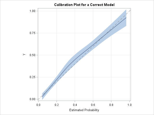
This calibration plot indicates that the quadratic model fits the data well. The calibration curve is close to the diagonal reference line, which is the line of perfect calibration. The curve indicates that the predicted and empirical probabilities are close to each other for low-risk, moderate-risk, and high-risk subjects.

It is acceptable for the calibration curve to have small dips, bends, and wiggles. The extent that the curve wiggles is determined by the (automatically chosen) smoothing parameter for the loess algorithm, The value of the smoothing parameter is not displayed by PROC SGPLOT, but you can use PROC LOESS to display the smoothing parameter and other statistics for the loess smoother.

According to Austin and Steyerberg (2013), the calibration curve can detect misspecified models when the magnitude of the omitted term (or terms) is moderate to strong. The calibration curve also behaves better for large samples and when the incidence of events is close to 50% (as opposed to having rare events). Lastly, there is a connection between discrimination and calibration: The calibration curve is most effective in models for which the discrimination (as measured by the C-statistic or area under the ROC curve) is good.

Summary

In summary, this article shows how to construct a loess-based calibration curve for logistic regression models in SAS. To create a calibration curve, use PROC LOGISTIC to output the predicted probabilities for the model and plot a loess curve that regresses the observed responses onto the predicted probabilities.

You can download the SAS code used in this article. My next article shows how to construct a popular alternative to the loess-based calibration curve, called a decile calibration plot. In the alternative version, the subjects are ranked into deciles according to the predicted probability or risk.

Update (20EB2019): If you have SAS/STAT 15.1 (SAS 9.4M6), you can create a calibration plot automatically by using PROC LOGISTIC.

Further reading

• Austin and Steyerberg (2013), "Graphical assessment of internal and external calibration of logistic regression models by using loess smoothers," Statistics in Medicine.
• Hosmer, Hosmer, Le Cessie, and Lemeshow (1997), "A comparison of goodness-of-fit tests for the logistic regression model," Statistics in Medicine.