At SAS Global Forum 2019, Daymond Ling presented an interesting discussion of binary classifiers in the financial industry. The discussion is motivated by a practical question: If you deploy a predictive model, how can you assess whether the model is no longer working well and needs to be replaced?
Daymond discussed the following three criteria for choosing a model:
- Discrimination: The ability of the binary classifier to predict the class of a labeled observation. The area under an ROC curve is one measure of a binary model's discrimination power. In SAS, you can compute the ROC curve for any predictive model.
- Accuracy: The ability of the model to estimate the probability of an event. The calibration curve is a graphical indication of a model's accuracy. In SAS, you can compute a calibration curve manually, or you can use PROC LOGISTIC in SAS/STAT 15.1 to automatically compute a calibration curve.
- Stability: Point estimates are often used to choose a model, but you should be aware of the variability of the estimates. This is a basic concept in statistics: When choosing between two unbiased estimators, you should usually choose the one that has smaller variance. SAS procedures provide (asymptotic) standard errors for many statistics such as the area under an ROC curve. If you have reason to doubt the accuracy of an asymptotic estimate, you can use bootstrap methods in SAS to estimate the sampling distribution of the statistic.
Estimates of model stability
My article about comparing the ROC curves for predictive models contains two competing models: A model from using PROC LOGISTIC and an "Expert model" that was constructed by asking domain experts for their opinions. (The source of the models is irrelevant; you can use any binary classifier.) You can download the SAS program that produces the following table, which estimates the area under each ROC curve, the standard error, and 90% confidence intervals:
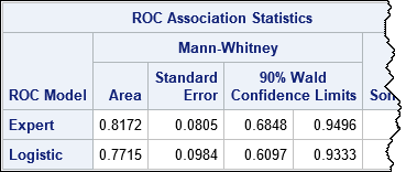
The "Expert" model has a larger Area statistic and a smaller standard error, so you might choose to deploy it as a "champion model."
In his presentation, Daymond asked an important question. Suppose one month later you run the model on a new batch of labeled data and discover that the area under the ROC curve for the new data is only 0.73. Should you be concerned? Does this indicate that the model has degraded and is no longer suitable? Should you cast out this model, re-train all the models (at considerable time and expense), and deploy a new "champion"?
The answer depends on whether you think Area = 0.73 represents a degraded model or whether it can be attributed to sampling variability. The statistic 0.73 is barely more than 1 standard error away from the point estimate, and you will recall that 68% of a normal distribution is within one standard deviation of the mean. From that point of view, the value 0.73 is not surprising. Furthermore, the 90% confidence interval indicates that if you run this model every day for 100 days, you will probably encounter statistics lower than 0.68 merely due to sampling variability. In other words, a solitary low score might not indicate that the model is no longer valid.
Bootstrap estimates of model stability
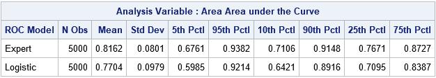
If "asymptotic normality" makes you nervous, you can use the bootstrap method to obtain estimates of the standard error and the distribution of the Area statistic. The following table summarizes the results of 5,000 bootstrap replications. The results are very close to the asymptotic results in the previous table. In particular, the standard error of the Area statistic is estimated as 0.08 and in 90% of the bootstrap samples, the Area was in the interval [0.676, 0.983]. The conclusion from the bootstrap computation is the same as for the asymptotic estimates: you should expect the Area statistic to bounce around. A value such as 0.73 is not unusual and does not necessarily indicate that the model has degraded.
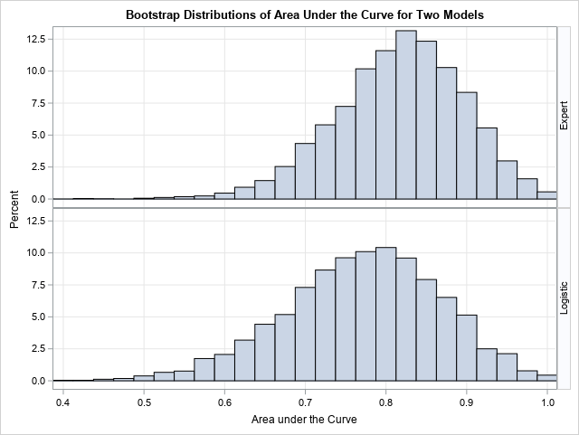
You can use the bootstrap computations to graphically reveal the stability of the two models. The following comparative histogram shows the bootstrap distributions of the Area statistic for the "Expert" and "Logistic" models. You can see that not only is the upper distribution shifted to the right, but it has less variance and therefore greater stability.
I think Daymond's main points are important to remember. Namely, discrimination and accuracy are important for choosing a model, but understanding the stability of the model (the variation of the estimates) is essential for determining when a model is no longer working well and should be replaced. There is no need to replace a model for a "bad score" if that score is within the range of typical statistical variation.
References
Ling, D. (2019), "Measuring Model Stability", Proceedings of the SAS Global Forum 2019 Conference.
Download the complete SAS program that creates the analyses and graphs in this article.

3 Comments
Using specific metrics to evaluate a predictive model on a given data set is not the same as using those metrics to compare the performance of that model on two or more distinct data sets.
The metrics are primarily useful for comparing the performance of two or more models on the SAME data set.
The metrics used may be dependent on the proportions of each binary category ( Good, Bad ) within the data set and as such if the two data sets that are used for the comparison have significantly different Good/Bad ratios then the use of these metrics may be misleading.
Hi, Jon. Thanks for writing. I'm not sure why you think there are two different data sets. My previous article has only one data set from which two different models are created. What you might have mistaken as a second "data set" is actually the sequence of 43 predicted values from the expert model, but those predictions are for the same set of 43 observations as the logistic model. Sorry if that was not clear.
Hi Jon, in practice, there are many comparisons of different models on different datasets. For example, comparing metrics of different models on a validation dataset to find the "best" model, or comparing metrics of a model on different validation datasets from different time periods to see if performance holds out of period. These are done to understand model performance/stability on known datasets.
There is another situation where one does not have control over the datasets, rather the task is to assess quality of different datasets. For example, you might have a credit portfolio and a trusted risk model, and you may be asked to evaluate the quality of another portfolio. To the extent you believe the model is reliable, you can compare the score distributions of the datasets to understand their relative quality. This is done to evaluate the risk of different credit portfolios all the time in practice.