I follow several data visualization experts on social media. Sometimes, I see a graph that I struggle to interpret. When that happens, I ask myself whether there is a simpler and more effective way to visualize the data. Recently, I saw an example of using a "horizon plot" to visualize decades of gas prices in the US. I didn't understand the graph. This article uses a "lasagna plot" to visualize the same data. The lasagna plot is a simpler and more effective visualization.

The horizon plot

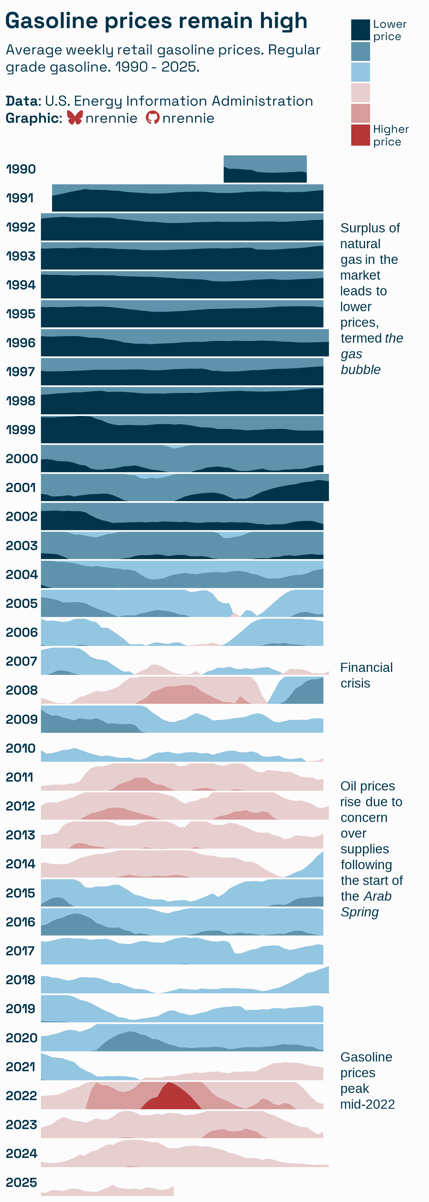
The graph shown to the right is an example of a horizon plot that was created and posted by Nicola Rennie, who is an accomplished data visualization designer, lecturer, and author. It was created to visualize the average price of gasoline in the US over several decades.

This was the first time I had ever seen a horizon plot. I didn't understand it. I had many questions:

• The graph shows gas prices, but what was the price of a gallon of gas at the beginning of 1993? What was the price at the beginning of 2025? In short, what is the scale of the vertical axis for each row?
• What does the horizontal axis represent? I assume it is time, but how can I discover the price of gas in October of 2008 by looking at the graph?
• The legend indicates that colors represent prices. What is the price range for each color? Why do some rows (years) have multiple colors? For example, the beginning of 1993 has a light-blue color on top of a dark-blue color.

Rennie included a link to a web page that explains how to construct and interpret a horizon plot. The web page claims that horizon plots are "frequently used in time-series data to represent a moving value." It claims that the value of the horizon plot is that it uses "a fraction of the vertical space" required by a standard line plot. To save vertical space, the plot uses a complex series of color-coding, reflections, and overplotting.

After reading the explanation, I now understand the plot. However, I don't like it and do not recommend it. I am an advocate of the adage, "simpler is better" for visualizing data. For these gas prices, I think a simple lasagna plot is a better choice.

A lasagna plot

A lasagna plot is a heat map. A lasagna plot is a useful alternative to a spaghetti plot, which overlays a set of line plots. When the line plots overlap substantially, it is difficult to read a spaghetti plot. A lasagna plot provides a simple alternative that is easier to read.

For the gas-price data, a lasagna plot is a matrix of colored cells:

• Each row shows one year of data.
• The horizontal axis represents time. By asking the author for the data, I discovered that the prices are weekly averages, so the horizontal axis should represent the weeks in a year. Most years have 52 weeks, but some have 53, so each row will contain either 52 or 53 cells. You can see this effect in the horizon plot, too. Notice that some weeks are longer than the surrounding years. There are several ways to assign weeks to dates. I used the ISO standard.
• The cells are colored. The color represents the average cost of gas for the year (row) and week (column).

Create a lasagna plot in SAS

The first step to creating a plot is to obtain the data. To keep the article focused on the graphics, I show only an overview of a SAS DATA step that can read Date and Price data. Rennie provided an XLS file that contains a column of dates and 12 columns of various gasoline prices. I'm not sure which column Rennie used, but I chose the column for Regular Gasoline that has the variable name EMM_EPMR_PTE_NUS_DPG. I simply downloaded the file, but Chris Hemedinger and the SAS documentation provide many examples of fetching data directly from the internet and importing it into a SAS data set.

You can use the ANYDTDTE. informat in SAS to read the column of dates. For each date, you can use the YEAR function to extract the year and the WEEK function to extract the week of the year. If the week is the first of last week of a year, you might have to adjust the YEAR variable to reflect the year to which the week belongs.

In the lasagna plot, the YEAR variable is used for the rows, the WEEK variable is used for the columns, and the PRICE variable is used for the color of each cell. Here is one way to read the data:

/* remake the "horizon plot" at https://github.com/nrennie/tidytuesday/tree/main/2025/2025-07-01
   from the data at https://github.com/rfordatascience/tidytuesday/blob/main/data/2025/2025-07-01/readme.md
*/
data GasPrices;
infile datalines missover;  /* handle missing values */
format Date DATE10.;
input @1 Date anydtdte12.   /* the ANYDTDTE format is great! */
      @13 Price;
Week = week(Date, 'V');     /* convert date into week of the year */
if Week=1 then 
   Year = year(Date+7);     /* is the week part of next year, last year, or this year? */
else if Week>=52 then 
   Year = year(Date-7);
else 
   Year = year(Date);
label Price = "US Regular Gasoline: Average Price ($/gal)";
datalines;
Aug 20, 1990	1.191
Aug 27, 1990	1.245
Sep 03, 1990	1.242
...<read data from 1990-2025>...
Jun 09, 2025	3.108
Jun 16, 2025	3.139
Jun 23, 2025	3.213
;

After reading the data, you can use the HEATMAPPARM statement in PROC SGPLOT to visualize the data. For an initial visualization, I've used the COLORMODEL= option to specify a two-color ramp, which assigns light-to-dark shades of blue colors to cells. This results in the following visualization:

/* make the graph long enough for 36 rows of cells */
ods graphics/ width=500px height=800px discretemax=10000;
/* use a sequential color ramp to show low-high variation */
title "US Gas Average Prices";
title2 "Regular Gas: 1990-2025";
proc sgplot data=GasPrices;
   format Price dollar5.2;
   heatmapparm x=Week y=Year colorresponse=Price / colormodel=TwoColorRamp;
   yaxis display=(nolabel) labelattrs=(size=6pt) reverse values=(1990 to 2025) fitpolicy=none;
   xaxis labelattrs=(size=8pt) values=(1 to 53 by 4);
run;

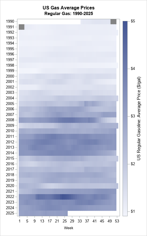
The lasagna plot is easy to understand. The two-color color ramp enables the viewer to estimate the price of gas at any time. Of course, graphs are designed to show trends and qualitative features, not exact prices. Nevertheless, you should be able to roughly estimate a price from a graph. For example, the price at the beginning of 1993 looks to be about $1.00-$1.20, based on the very light (almost white) color of that cell. To find the price in October of 2008 requires knowing where to look. October is the tenth month, so you should look at the cells for weeks 40-45. It looks like there was a rapid transition of prices during that month. The price fell from $3.50 to (maybe) $2.50? It is hard to tell because the graph uses similar shades of the same color.

Although exact prices are difficult to discern, the lasagna plot clearly shows the highs, lows, and trends for prices of regular gas from 1990 to 2025:

• The years 1990-2000 were characterized by relatively low and steady gas prices.
• The price became more expensive in the 2000s, culminating in the financial crisis of 2007-2008.
• A glut of oil production led to low prices in 2015.
• The COVID pandemic in 2020 led to low demand and low prices.
• Russia invaded Ukraine on 24 February 2022, which higher prices of oil on the world market.

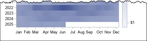
Depending on how the graph will be used, you might want to replace the tick marks for the weeks with text for Jan, Feb, ..., Dec. You can use the VALUESDISPLAY= option on the XAXIS statement to accomplish that. I leave the details as an exercise, but the result is a nonuniform placement of ticks, as follows.

Sequential versus diverging color ramps

The previous section shows a lasagna plot that uses a two-color sequential color ramp. Using shades of a single color can make it hard to estimate values. The original horizon plot of these data used more colors: shades of red for high prices and shades of blue for low prices. You can use a diverging red-blue palette of colors on the COLORMODEL= option to achieve a similar effect for the lasagna plot. In a three-color diverging ramp, the midrange of the data (about $3 per gallon) is represented by a third color, which is off-white. This corresponds to the "horizon" in a horizon plot.

/* use a diverging color ramp to show deviations from a baseline such as $3 / gal */
%let DivRedBlueModel = (CX2166AC CX67A9CF CXD1E5F0 CXFDDBC7 CXEF8A62 CXB2182B);
proc sgplot data=GasPrices;
   format Price dollar5.2;
   heatmapparm x=Week y=Year colorresponse=Price / colormodel=&DivRedBlueModel;  /* change the color model */
   yaxis display=(nolabel) labelattrs=(size=6pt) reverse values=(1990 to 2025) fitpolicy=none;
   xaxis labelattrs=(size=8pt) values=(1 to 53 by 4);
run;

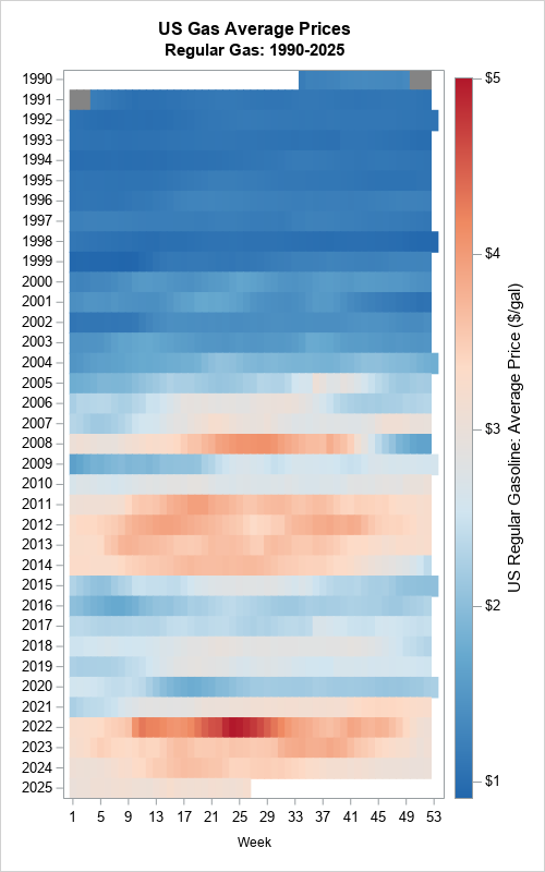
With this three-color ramp, it is easier to estimate prices from colors. For example, in October of 2008, the drop from $3.50 to $2.50 per gallon is easier to estimate.

Summary

The goal of data visualization is to create a graph that effectively conveys important features of the data. Statistical software enables you to create many fancy graphs. But if your goal is effective communication, "fancier" is not always better. This article shows two visualizations of a time series of US gasoline prices. The first is a horizon plot, which is a non-standard plot that can be confusing if you have never seen it before. In contrast, a lasagna plot is easier to understand and interpret. The lasagna plot is a heat map of the data arranged in rows and columns.