A course in elementary statistics always introduces the "Z-score." A Z-score is the result of standardizing a normally distributed random variable. By subtracting the distribution's mean and dividing by its standard deviation, you transform a general normal random variable into a standardized variable that has zero mean and unit standard deviation. Historically, this transformation was essential because it enabled statisticians to look up probabilities in a single printed table. Conceptually, it enables a uniform analysis of normally distributions by measuring all quantities in units of the standard deviation about the mean.
The concept of a "Z-score" also applies to multivariate normal distributions. In multidimensional statistics, you can standardize a multivariate normal (MVN) probability calculation by transforming the covariance matrix into the corresponding correlation matrix. This article shows how to shift and scale high-dimensional MVN distributions, both mathematically and by using the SAS IML language.
The 1-D Z-score transformation
Let's start by reviewing the Z-score transformation for the 1-D normal distribution. Let X be a normally distributed random variable with mean μ and standard deviation σ. In notation, X ∼ N(μ, σ). (Some authors use N(μ, σ2), but the SAS probability functions (CDF, PDF, QUANTILE, etc.) use the standard deviation as a parameter.) If you want to compute a left-tail probability, such as P(X < b), you can compute the probability on the original (data) scale, or you can apply a transformation and compute the probability on the standardized scale. This is useful in numerical computations because it reduces the problem to two steps: first, standardize the problem, then compute a probability on the standardized problem. Each of these steps can be developed, debugged, and tested independently.
Let's apply the Z-score transformation. Define a new random variable Z = (X - μ)/σ. Because a linear transformation of a normal random variable is also normal, Z follows a standard normal distribution: Z ∼ N(0, 1).
By applying the same transformation to the integration limit b, we define a standardized limit c = (b - μ)/σ. Consequently, computing the probability on the original data scale is mathematically equivalent to computing the probability on the standardized scale:
P(X < b | X~N(μ, σ)) = P(Z < c | Z~N(0, 1))
In SAS, you can compute these probabilities directly using the CDF function.
The following SAS IML program demonstrates this equivalence.
The goal is to find the probability that a random variable from N(μ, σ) is less than x.
You can compute this directly on the original scale, or you can convert the
limit to a Z-score and evaluate it using the standard normal distribution:
data Prob; input mu sigma @@; do x = -1 to 1; /* 1. Compute probability on original scale */ prob_x = CDF("Normal", x, mu, sigma); /* 2. Compute probability on standardized scale */ z = (x - mu)/sigma; prob_z = CDF("Normal", z); /* N(0,1) */ output; end; datalines; 2 3 1.5 2 -0.5 0.5 run; proc print noobs; run; |
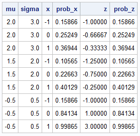
The program uses several examples of x, μ and σ. For all examples, the PROB_X and the PROB_Z columns are identical. Geometrically, the X variable represents a data value whereas the Z variable measures the number of standard deviations from the mean. As shown in the next section, you can generalize this concept to multivariate normal distributions.
Standardizing the multivariate normal distribution
Suppose you want to compute the joint cumulative probability for a multivariate normal distribution. Let X be a k-dimensional random variable such that X ∼ MVN(μ, Σ), where μ = (μ1, μ2, ..., μk) is the mean vector and Σ is a k x k covariance matrix. The CDF or left-tail probability is P(X < b), where b = (b1, b2, ..., bk) is a vector of upper limits, and the inequality is evaluated component by component.
To standardize this problem, you can standardize each original variable. Instead of doing this one variable at a time, you can use matrix-vector notation and transform all variables simultaneously. Let D be the diagonal matrix of standard deviations. That is, the diagonal elements of D are the square roots of the diagonal elements of Σ. Then you can express the covariance matrix as Σ = D*R*D, where the matrix R has 1s on the diagonal. The matrix R is the correlation matrix for the original variables (and the covariance matrix for the new standardized variables).
The standardized random variables are defined by Z = D-1(X - μ). Z is multivariate normal. To find its parameters, you can compute its expected value and variance. The expected value is simply a vector of zeros. The variance of Z is R. Thus, the transformed variable Z follows a standardized multivariate normal distribution with mean zero and correlation matrix R. In notation, Z ~ MVN(0, R).
To complete the probability transformation, apply the same linear transformation to the integration limits, b.
The standardized limits are c = D-1(b - μ).
A probability for X on the data scale (covariance scale) is equal to the probability for Z on the correlation scale:
P(X < b | X ~ MVN(μ, Σ)) = P(Z < c | Z ~ MVN(0, R))
This is why, for example, the PROBBNRM function in SAS computes probabilities for the standardized variable Z~BVN(0, R), where BVN is the bivariate normal distribution, and R is a 2x2 correlation matrix. The developer who implemented the function assumed that users can transform any problem to the standardized scale.
Converting from covariance to correlation in SAS IML
The SAS IML language supports the COV2CORR function, which returns the correlation matrix that is associated with a covariance matrix. By using the math in the previous section, you can write a SAS IML function that will transform the limits of integration. The following IML function computes c = D-1(b - μ). The SAS IML language enables you to perform this operation efficiently by using vectorized division, rather than multiplying by the inverse of a diagonal matrix:
proc iml; /* Sigma is a kxk covariance matrix and b is a row vector with k elements. Convert b to inv(D)*(b-mu), where D is the diagonal matrix of standard deviations: sqrt(vecdiag(Sigma)). The mu vector is optional and defaults to the zero vector. */ start Xform_Limits_Cov2Corr( b, Sigma, mu=j(1,ncol(Sigma),0) ); D = sqrt(vecdiag(Sigma)); /* extract diagonal (variances) for X */ c = (b - mu) / rowvec(D); /* new limits for Z */ return c; finish; |
As we did for the 1-D case, let's show the equivalency between the CDF on the data scale and the CDF for the standardized problem. The exact computation of multivariate normal probabilities in high dimensions is difficult. Instead, I will use a simple Monte Carlo simulation to estimate the probabilities. This technique is easy to code and will suffice to demonstrate the equivalency of the probabilities.
/* Use Monte Carlo simulation to estimate the probability that a MVN random variable is less than a specified value in each coordinate. Sigma is a kxk covariance matrix; mu is an optional row vector with k elements. The row vector b specifies the upper limits of integration. The function returns an estimate of P(X1<b[1] & X2<b[2] & ... & Xk<b[k] | X~MVN(mu, Sigma)) by simulating N random variates from MVN(mu, Sigma) and returning the proportion that are in the specified region. */ start MC_CDFMVN(N, b, Sigma, mu=j(1,ncol(Sigma),0)); X = randnormal(N, mu, Sigma); inRegion = j(N, 1, 1); do i = 1 to ncol(b); v = (X[,i] < b[i]); /* binary variable for the i_th coordinate */ inRegion = inRegion & v; /* find the intersection of all conditions */ end; return mean(inRegion); /* proportion of random points that satisfy criterion */ finish; |
An Example: The 5-D Min Matrix
You can use the built-in COV2CORR function and the newly defined Xform_Limits_Cov2Corr function to
transform a problem on the covariance (data) scale into an equivalent standardized problem.
We will use a 5-dimensional "Min Matrix" as our covariance matrix. The Min Matrix is a structured matrix where the (i, j)-th element is equal to min(i, j).
The mean vector, μ, and the integration limits, b, are arbitrary vectors.
The following program estimates the probability twice, both times using one million random variates in a Monte Carlo simulation.
First, it uses the MC_CDFMVN function for the 5-D Min Matrix.
Then it transforms the limits, creates the associated correlation matrix, and estimates the probability on the standardized scale.
So that the estimates are the same, and not just close to each other, you can use the RANDSEED subroutine
to reset the random number stream prior to each simulation. This ensures that both computations use the exact same stream of pseudo-random numbers.
/* Example: use a 5-D "Min Matrix". See: https://blogs.sas.com/content/iml/2026/02/16/min-matrix.html */ /* Define the parameters for MVN(mu, Sigma) */ Sigma = {1 1 1 1 1, 1 2 2 2 2, 1 2 3 3 3, 1 2 3 4 4, 1 2 3 4 5 }; mu = {1 2 3 4 5}; N = 1E6; /* estimate the CDF probability at b for MVN(mu, Sigma)*/ b = {-1 2 2 3 7}; call randseed(1234, 1); /* reset the RNG */ prob_cov = MC_CDFMVN(N, b, Sigma, mu); /* standardize the parameters to the correlation scale */ c = Xform_Limits_Cov2Corr(b, Sigma, mu); R = cov2corr(Sigma); /* estimate the CDF probability at c for MVN(0, R)*/ call randseed(1234, 1); /* reset the RNG */ prob_corr = MC_CDFMVN(N, c, R); print prob_cov prob_corr; |
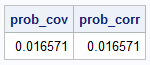
The output shows that the probability estimate for the original problem is identical to the estimate for the standardized problem.
Summary
You can use techniques from linear algebra to extend the concept of a Z-score to multivariate normal distributions. You do not have to physically standardize each column of the data. Rather, you can convert the covariance matrix to the associated correlation matrix, apply a linear transformation to the limits of integration, and—voilà!—you can compute all multivariate normal probabilities in a standardized way.
This transformation is not purely academic. In computational statistics, algorithms that evaluate multivariate distributions are often implemented for the standardized correlation scale to ensure stable numerical computations. By scaling the problem and then computing answers on the correlation scale, the numerical routines tend to be more accurate and reliable.
