Properties of the "Min Matrix"

When you implement a numerical algorithm, it is helpful to write tests for which the answer is known analytically. Because I work in computational statistics, I am always looking for test matrices that are symmetric and positive definite because those matrices can be used as covariance matrices. I have previously written about some useful test matrices:

The Pascal matrix is a symmetric positive definite matrix with a known Cholesky decomposition and inverse.
A Toeplitz matrix is symmetric (and banded) and can be constructed so that it is positive definite.
A special Toeplitz matrix, called the first-order autoregressive (AR(1)) correlation matrix, has explicit eigenvalues.

I recently learned about another symmetric and positive definite matrix, called the Min Matrix. The Min Matrix of size n is the matrix defined by M[i,j] = min(i,j) for 1 ≤ i,j ≤ n. The general form of the Min Matrix is shown below:

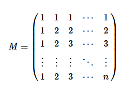
The Min Matrix has some wonderful properties. It is easy to generate. It is symmetric and positive definite (SPD). The inverse and Cholesky roots are also integer valued. The eigenvalues have explicit formulas.

Creating the Min Matrix in SAS IML

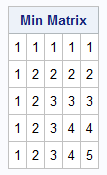
In the SAS IML language, you can create the Min Matrix without using any loops. By using the built-in ROW and COL functions in conjunction with the elementwise minimum operator (><), you can generate the matrix in a single line of code:

proc iml;
/* return the Min Matrix of size n. M[i,j] = min(i,j) */
start MinMatrix(n);
   M = row(I(n)) >< col(I(n));
   return M;
finish;
 
n = 5;
M = MinMatrix(n);
print M[L='Min Matrix'];

The Cholesky root and the determinant

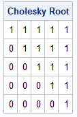
A property of the Min Matrix is that its Cholesky factor is known and integer-valued. The Cholesky root of an SPD matrix, M, is an upper-triangular matrix, U, such that M = U^TU. (In PROC IML, the ROOT function returns the upper triangular factor.) For the Min Matrix, the Cholesky root contains all 1s on and above the main diagonal. Not only is this a cool result, but the root immediately tells us that the determinant of M is always 1. This follows because det(M) = det(U^T)det(U) = 1.

U = root(M);
print U[L='Cholesky Root'];

The tridiagonal inverse

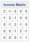
The Min Matrix is a dense matrix, but its inverse is a tridiagonal matrix. The inverse matrix has 2s on the main diagonal (except for the very last element, which is 1) and -1s on the superdiagonal and subdiagonal. This inverse matrix is closely related to the matrix for a discrete second-difference operator, except for the (n,n)th element.

M_Inv = inv(M);
print M_Inv[L='Inverse Matrix'];

Eigenvalues

The structure of the inverse matrix enables use to find a formula for its eigenvalues. The k_th eigenvalue for M^-1 is $\mu_k = 4 \sin^2\left( \frac{(2k-1)\pi}{2(2n+1)} \right)$

For any invertible matrix, the eigenvalues of the matrix and its inverse are reciprocals. Therefore, the eigenvalues of the Min Matrix of size n are given by the following expression: $\lambda_k = \frac{1}{4 \sin^2\left( \frac{(2k-1)\pi}{2(2n+1)} \right)}$

You can verify this formula by comparing the analytical results to the numerical computation from the EIGVAL function:

eigenvals = eigval(M);    /* numerical eigenvalues */
/* compare to the analytical formula */
k = T(1:n);
pi = constant('pi');
check_eig = 1 / (4 * sin( ((2*k-1)*pi) / (2*(2*n+1)) )##2);
Diff = eigenvals - check_eig;
print eigenvals check_eig Diff;

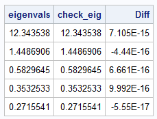
From the analytical expression for the eigenvalues, you can deduce that the Min Matrix is ill-conditioned for large n. As n increases, the largest eigenvalue (k=1) grows like O(n²). In contrast, the smallest eigenvalue (k=n) approaches the value 1/4. The condition number of a matrix is the ratio of the largest to smallest eigenvalue, so the condition number of the Min Matrix grows quadratically with n. This makes it an a good test case for matrix computations.

Summary

The Min Matrix is a good test matrix to know about. It is a covariance matrix because it is symmetric and positive definite. It is easy to construct, it has a simple Cholesky root, it has an integer-valued tridiagonal inverse, and its eigenvalues are known exactly.

Blogs