The first-order autoregressive (AR(1)) correlation structure is important for applications in time series modeling and for repeated measures analysis. The AR(1) model provides a simple situations where measurements (on the same subject) that are closer in time are correlated more strongly than measurements recorded far apart. The AR(1) model uses a single parameter, ρ, to represent the correlation between consecutive measurements. The (i,j)th element of the n x n covariance matrix has the form σ2 ρ|i-j| for i,j = 1..n. Similarly, the (i,j)th element of the correlation matrix is ρ|i-j|.
The covariance (and correlation) matrix of an AR(1) process are specific instances of a Toeplitz matrix because the matrix is constant along each diagonal, including sub- and super-diagonals. This current article shares a result of Peter J. Sherman (2023, IEEE Statistical Signal Processing Workshop) who published formulas for the eigenvalues and vectors of an AR(1) covariance matrix. His paper is behind a pay wall, but this article provides a summary of the most important formulas. You can download the complete SAS program that creates all tables and graphs in this article.
Explicit formulas for eigenvalues are rare
As I have written previously, not many matrices have an explicit formula for eigenvalues. This is because eigenvalues are the roots of a high-order polynomial, and Galois theory proves that there is no general formula for high-order polynomials in terms of radicals (square roots, cube roots, etc). However, there are exceptions for classes of matrices that contain a lot of structure. For example, I have previously showed that there is an explicit formula for the eigenvalues of a tridiagonal Toeplitz matrix.
Sherman (2023) shows another example: an AR(1) covariance matrix has so much structure that the roots of its characteristic polynomial can almost be written exactly in terms of a formula. The formula is almost—but not quite—exact because the formula involves one quantity that must be completed numerically by solving for the root of one-dimensional function on a closed interval. However, this step is easy to program. For that reason, I call the formula "explicit" rather than "exact."
The eigenvalues of an AR(1) correlation matrix
Without loss of generality, we can consider the n x n AR(1) correlation matrix, R. That is because the covariance matrix, S, is of the form S = σ2 R, and if (λ, v) is an eigenpair for R then (σ2λ, v) is an eigenpair for S. In the following, references such as [Eqn 1] refer to the equation numbers in Sherman (2023). Equations 1-2 appear on p. 6; equations 5-8 appear on p. 7.
The eigenvalues are ultimately defined in terms of the roots of the following rational trigonometric function [Eqn 2]:
\(P_n(\omega) =
\left(
\sin((n+1)\omega) - 2\rho\sin(n\omega)+\rho^{2}\sin((n-1)\omega)
\right) / \sin(\omega)
\)
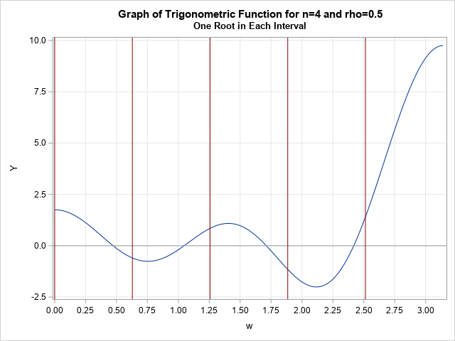
The function Pn has n roots on the interval [0, π]. The k_th root of the function, which we call ωk, is in the interval
(ak-1, ak), where ak = k π / (n+1).
The following graph shows the function for n=4 and ρ=0.5. The first root is in the interval (0, π/5), the second root is in the interval (π/5, 2π/5),
and so forth, until the last root, which is in the interval (3π/5, 4π/5)
The function Pn has a removeable singularity at ω = 0, so you can define the value Pn(0) to be
the limiting value (n+1) – 2nρ + (n-1)ρ2.
Most numerical packages include an easy way numerically approximate of the root of the function on each interval. In SAS IML, you can use the FROOT function.
In terms of the k_th root, ωk, the k_th eigenvalue of R is [Eqn 1]
\( \lambda_k = (1 - \rho^2) / (1 - 2 \rho\cos(w_k) + \rho^2 )\)
A program for the eigenvalues of an AR(1) correlation matrix
The following SAS IML program defines a function, SineRational, that evaluates the rational trig function. The function GetSineRationalRoots calls the FROOT function to find roots of the function. The function EigenvalsAR1 uses the roots to return the complete set of eigenvalues. By default, these functions find all roots and all eigenvalues. However, as I will discuss later, the last argument enables you to specify a subset of the root and eigenvalues.
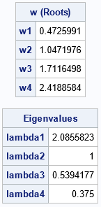
proc iml; /* Eqn 1: Define the rational trig function that avoids the undefined value at w=0 */ start SineRational(w, rho, n); if w=0 then return (n+1) -2*rho*n + rho##2*(n-1); p = sin( (n+1)*w ) -2*rho*sin(n*w) + rho##2*sin((n-1)*w); return( p / sin(w) ); finish; /* A one-variable version of the rational trig function; put parameters into GLOBAL clause */ start SineRationalFun(w) global( g_rho, g_dim ); return( SineRational(w, g_rho, g_dim) ); finish; /* Get the k_th roots of a rational trig function. By default, get all eigenvalues when seq=1:n. The last arg determines a subset of roots. For example, 1:3 will get the first 3 roots. */ start GetSineRationalRoots(rho, n, seq=1:n) global( g_rho, g_dim ); g_rho = rho; g_dim = n; /* copy parameters to global vars */ pi = constant('pi'); endpts = (0:n)*pi / (n+1); intervals = endpts[1:n] || endpts[2:(n+1)]; intervals = intervals[seq,]; /* get only the specified roots */ roots = froot("SineRationalFun", intervals); return roots; finish; /* Get eigenvalues of an (n x n) AR1(rho) matrix. By default, get all eigenvalues 1:n. Specify the last arg to get only a subset. For example, 1:3 will get only the top 3. */ start EigenvalsAR1(rho, n, seq=1:n); w = GetSineRationalRoots(rho, n, seq); lambda = (1-rho##2) / (1 - 2*rho*cos(w) + rho##2); return lambda; finish; /* Example: find roots and eigenvalues for n=4 and rho=0.5 */ n = 4; rho = 0.5; w = GetSineRationalRoots(rho, n); print w[L="w (Roots)" r=('w1':'w4')]; eval = EigenvalsAR1(rho, n); print eval[L="Eigenvalues" r=('lambda1':'lambda4')];; |
You can explicitly form the AR(1) correlation matrix, call the EIGVAL function, and verify that the eigenvalues obtained by using the explicit formulas are the same as the eigenvalues obtained by conventional numerical methods.
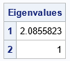
The previous example finds all n eigenvalues. However, the program supports an optional last argument, called SEQ, that you can use to specify a subset of the eigenvalues. This can be useful, for example, if you want to compute only the first few or the last few eigenvalues. For example, if you want only the first two eigenvalues, specify the values 1:2 for the last parameter, as follows:
/* Example 2: find only top two eigenvalues */ seq = 1:2; eval2 = EigenvalsAR1(rho, n, seq); print eval2[L="Eigenvalues" r=seq]; |
The eigenvectors of an AR(1) correlation matrix
Sherman's paper also shows formulas for the k_th eigenvector of the AR(1) covariance or correlation matrix. Again, the computation relies on the
numerical roots of the function Pn.
It also requires two auxiliary constants, for the k_th eigenvector, define the constant [Eqn 8]
\(
c_k = \sqrt{1 - 2 \rho\cos(w_k) + \rho^2 }
\)
and define the phase angle [Eqn 6] as
\(
\phi_k = \tan^{-1}\left(
\frac{\rho \sin(\omega_k)}
{1 - \rho \cos(\omega_k)}
\right)
\)
With those constants defined, the k_th eigenvector of R is the following column vector [Eqn 5]:
\(
v_k = c_k \begin{bmatrix}
\sin(\omega_k + \phi_k), \sin(2\omega_k + \phi_k), \dots, \sin(n \omega_k + \phi_k)
\end{bmatrix}
\)
Sherman notes that these equations "are not well known among scientists and engineers who are involved with MA(1) and AR(1) processes" (p. 7).
A program for the eigenvectors of an AR(1) correlation matrix
The following SAS IML program defines two helper functions that evaluate the constants ck and φk for all k=1..n. The function EigenvectorsAR1 computes the roots of the Pn function and uses the constants to build a matrix whose columns are the formulas for the eigenvectors:
/* helper functions to return constants for the eigenvector formulas */ start GetPhi(w, rho); return atan( rho*sin(w) / (1 - rho*cos(w)) ); finish; start GetC(w, rho); return sqrt(1 - rho*cos(w) + rho##2); finish; /* Return the eigenvectors of an (n x n) AR(1) correlation matrix. By default, get all n eigenvectors. Specify the last arg to get only a subset. For example, 1:3 will get only the top 3. */ start EigenvectorsAR1(rho, n, seq=1:n); w = GetSineRationalRoots(rho, n, seq); w = rowvec(w); /* change to row vector */ phi = GetPhi(w, rho); c = GetC(w, rho); /* use the outer product to form matrix where columns are eigenvectors */ theta = T(1:n) * w + phi; return( c # sin( theta ) ); finish; /* Example: compute eigenvalues for n=4 */ evec = EigenvectorsAR1(rho, n); print evec[c=('v1':'v4')]; |
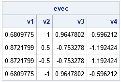
These are, in fact, eigenvectors of R, which you can verify by checking that the matrix A*evec - eval`#evec is the zero matrix.
Recall that eigenvectors are not unique: If v is an eigenvector for any matrix, then so is αv for any nonzero value of α. Thus, if you compare the eigenvectors that are formed by using Sherman's formulas to those computed by conventional methods, you must use ensure that all vectors have the same standardization. In SAS IML, the convention is that the eigenvectors have unit length. I used CALL EIGEN in PROC IML to compute the eigenvectors of the same 4 x 4 AR(1) matrix. The eigenvectors produced by the formulas agree with the conventional eigenvectors provided that you standardize the eigenvectors and ensure that they point in the same direction.
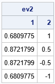
You can specify the last parameter to obtain only a subset of the eigenvectors, for example, if you want only the first two eigenvectors, use the following syntax:
/* Example: find only top two eigenvectors */ seq = 1:2; ev2 = EigenvectorsAR1(rho, n, seq); print ev2[c=seq]; |
Why is this result important?
Since we can already use numerical methods to find the eigenvalues and eigenvectors of any square matrix, why are the results in Sherman (2023) important?
- General-purpose numerical methods require that you store the entire n x n matrix. If you use the formulas, you do not need to store the matrix, only the parameter, ρ, and the size, n.
- Traditional eigenvalue solvers compute all n eigenvalues and eigenvectors, which is expensive. This method can compute any combination of eigenvalues, such as the five biggest or the three smallest.
- This method should handle values of ρ that are close to 0 or 1. Conventional methods might struggle with these limiting cases because the eigenstructure becomes degenerate.
Summary
Let R be the n x n AR(1) correlation matrix for the parameter ρ. That is, R[i,j] = ρ|i-j|. The explicit formulas in Sherman (2023) enable you to compute the k_th largest eigenvalue and eigenvector for k=1..n. The formulas are not exact because they require the numerical solution of the root of a rational trigonometric function, but they are fast, accurate, and do not require forming the R matrix.
You can download the complete SAS program that creates all tables and graphs in this article. The program also compares the eigenvalues and eigenvectors with conventional calls to CALL EIGEN in PROC IML.
References
This article is based on the formulas in Sherman (2023). The full reference is
P. J. Sherman, "On the Eigenstructure of the AR(1) Covariance," 2023 IEEE Statistical Signal Processing Workshop (SSP), Hanoi, Vietnam, 2023, pp. 6-10.
