Implement the generalized extreme value distribution in SAS

SAS supports more than 25 common probability distributions for the PDF, CDF, QUANTILE, and RAND functions. If you need a less-common distribution, you can implement new distributions by using Base SAS (specifically, PROC FCMP) or the SAS/IML language. On the SAS Support Communities, a SAS programmer asked how to implement the generalized extreme value (GEV) distribution in SAS. This article shows how to use PROC FCMP and PROC IML to implement functions for working with the GEV distribution.

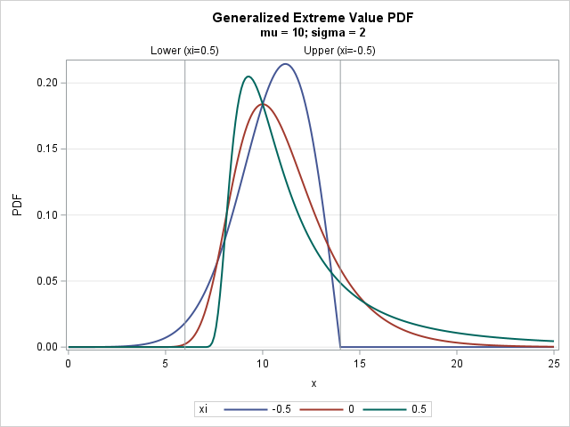
The density functions for three parameter values of the GEV distribution are shown to the right. The next section explains how the positive, negative, and zero values of the ξ parameter enable the GEV distribution to model multiple extreme-value distributions.

The generalized extreme value distribution

The Wikipedia article about the generalized extreme value distribution explains why the distribution is useful and provides all the formulas used in this article. Briefly, an "extreme value" distribution is one that describes the distribution of an extreme value such as the maximum (or minimum) of a different distribution. For example, the Gumbel distribution models the distribution of the maximum value in a sample n that is drawn from the standard normal distribution. But the Gumbel distribution is not the only way to model extreme events. The correct model depends on the heaviness or lightness of the tails of the data:

If a sample is drawn from a distribution that has light or medium tails (such as normal or lognormal), the distribution of the sample maximum can be modeled by using the Gumbel distribution.
If a sample is drawn from a distribution that has heavy tails (such as a t distribution), the distribution of the sample maximum can be modeled by using the Fréchet distribution. A heavy-tailed distribution decays according to a power law, which is slower than exponential decay.
If a sample is drawn from a distribution that has a finite upper bound (such as uniform or beta distribution), the distribution of the sample minimum can be modeled by using the Weibull distribution. Equivalently, the Weibull distribution models the maximum of -X.

These three models for extreme events can be combined into one super-duper distribution, known as the generalized extreme value distribution. The GEV(μ, σ, ξ) distribution has three parameters. The parameter μ is a location parameter; the parameter σ is a scale parameter. The parameter ξ (the Greek letter, xi) switches between the three previous distributions. For ξ < 0, the GEV corresponds to the (flipped) Weibull. For ξ = 0, the GEV corresponds to the Gumbel. For ξ > 0, the GEV corresponds to the Fréchet distribution.

Look back at the PDF of the GEV distribution at the top of this article. You can see that the PDF for ξ > 0 (the green curve), has a long right tail, as you would expect for a model of the maximum in heavy-tailed data.

Essential functions for the GEV Distribution

To work with a probability distribution, you need four essential functions: The CDF (cumulative distribution), the PDF (probability density), the QUANTILE function (inverse CDF), and a way to generate random values from the distribution. Each of these functions has an explicit formula for the GEV distribution, which are given in Wikipedia. However, the support of the PDF depends on the value of the shape parameter, ξ.

When ξ < 0, the support of the PDF is {x | x < μ – σ/ξ}. See the blue curve in the graph at the top of this article, whose support is x > 10 – 2/0.5 = 6. Equivalently, if you standardize the data by using z = (x – μ)/σ, then the support is {z | z < -1/ξ}.
When ξ = 0, the support of the PDF is the entire real line. See the red curve in the graph at the top of this article.
When ξ > 0, the support of the PDF is {x | x > μ – σ/ξ}. See the green curve in the graph, whose support is x < 10 – 2/(-0.5) = 14. Equivalently, if you standardize the data by using z = (x – μ)/σ, then the support is {z | z > -1/ξ}.

The following call to PROC FCMP defines four functions: CDF_GEV, PDF_GEV, QUANTILE_GEV, and RAND_GEV. The RAND_GEV generates a random uniform variate in (0,1), then calls the QUANTILE_GEV function to obtain a random GEV variate. This is known as the inverse CDF method for generating random variates.

/**********************************/
/* Define GEV functions in PROC FCMP. For details, see
   https://blogs.sas.com/content/iml/2012/04/18/extending-sas-how-to-define-new-functions-in-proc-fcmp-and-sasiml-software.html
 
   All GEV formulas are from https://en.wikipedia.org/wiki/Generalized_extreme_value_distribution */
proc fcmp outlib=work.funcs.ProbDist;
 
function CDF_GEV(x, mu, sigma, xi);
   if sigma <= 0 then return(.);
   /* support for x depends on mu - sigma/xi, so support for z depends on -1/xi */
   z = (x-mu)/sigma;
   if xi=0 then                            
      CDF = exp(-exp(-z));                 
   else if xi > 0 then do;
      if z > -1/xi then 
         CDF = exp(-(1 + xi*z)**(-1/xi));
      else 
         CDF = 0;
   end;
   else do; /* xi < 0 */
      if z < -1/xi then 
         CDF = exp(-(1 + xi*z)**(-1/xi));
      else 
         CDF = 1;
   end;
   return (CDF);
endsub;
 
function PDF_GEV(x, mu, sigma, xi);
   if sigma <= 0 then return(.);
   z = (x-mu)/sigma;
   if xi=0 then do;
      t = exp(-z);
      PDF = t**(xi+1) * exp(-t) / sigma;
      end;
   else if xi > 0 then do;
      if z > -1/xi then do;
         t = (1 + xi*z)**(-1/xi);
         PDF = t**(xi+1) * exp(-t) / sigma;
         end;
      else 
         PDF = 0;
   end;
   else do; /* xi < 0 */
      if z < -1/xi then do;
         t = (1 + xi*z)**(-1/xi);
         PDF = t**(xi+1) * exp(-t) / sigma;
         end;
      else 
         PDF = 0;
   end;
   return (PDF);
endsub;
 
function Quantile_GEV(p, mu, sigma, xi);
   if sigma <= 0 then return(.);
   if p<=0 | p>=1 then return(.);
   mLp = -log(p);
   if xi=0 then 
      x = mu - sigma*log(mLp);
   else 
      x = mu + sigma/xi*(mLp**(-xi) - 1);
   return (x);
endsub;
 
function Rand_GEV(mu, sigma, xi);
   p = rand("Uniform");
   x = Quantile_GEV(p, mu, sigma, xi);
   return (x);
endsub;
run;

Calling the FCMP functions

The previous section defined four functions by using PROC FCMP. This section shows how to call each one from the DATA step. First, you must use the CMPLIB= option to tell the DATA step where to find the functions. Let's start by calling the CDF_GEV function, which computes the CDF function for μ=10, σ=2, and for three values of ξ: ξ = -0.5, 0, and 0.5. You can use PROC SGPLOT to visualize the CDF curves, as follows:

options cmplib=work.funcs;  /* define location of GEV functions so the DATA step can find them */
%let mu = 10;               /* location parameter */
%let sigma = 2;             /* scale */
 
data CDF_Test;
mu = &mu;
sigma = &sigma;
dx = 0.1;
do xi = -0.5, 0, 0.5;    /* loop over three values of xi */
   do x = 0 to 25 by dx;
      CDF = CDF_GEV(x, mu, sigma, xi);
      output;
   end;
end;
run;
 
title "Generalized Extreme Value CDF";
title2 "mu = &mu; sigma = &sigma";
proc sgplot data=CDF_Test;
   series x=x y=CDF / group=xi lineattrs=(thickness=2);
   yaxis grid min=0 max=1;
   refline 6 14 / axis=x label=('Lower (xi=0.5)' 'Upper (xi=-0.5)');
run;

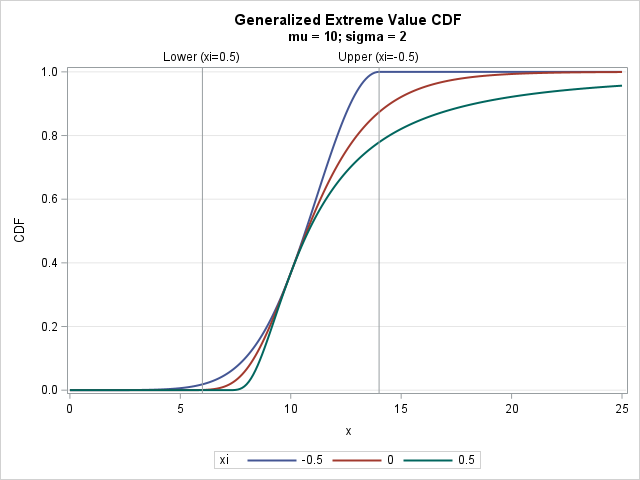
The graph includes a vertical reference line at x=6 for ξ = 0.5 (the green curve). For x < 6, the CDF is exactly 0. The graph also includes a vertical reference line at x=14 for ξ = -0.5 (the blue curve). For x > 6, the CDF is exactly 1.

In a similar way, you can call the PDF_GEV function in the DATA step. You can use PROC SGPOT to visualize the PDF functions:

data PDF_Test;
mu = &mu;
sigma = &sigma;
dx = 0.1;
do xi = -0.5, 0, 0.5;    /* loop over three values of xi */
   do x = 0 to 25 by dx;
      PDF = PDF_GEV(x, mu, sigma, xi);
      output;
   end;
end;
run;
 
title "Generalized Extreme Value PDF";
title2 "mu = &mu; sigma = &sigma";
proc sgplot data=PDF_Test;
   series x=x y=PDF / group=xi lineattrs=(thickness=2);
   yaxis grid;
   refline 6 14 / axis=x label=('Lower (xi=0.5)' 'Upper (xi=-0.5)');
run;

The graph is shown at the top of this article.

In a similar way, you can call the QUANTILE_GEV function in the DATA step. The domain of the quantile functions is the open interval (0, 1). You can use PROC SGPOT to visualize the quantile functions:

data Quantile_Test;
mu = &mu;
sigma = &sigma;
dp = 0.005;
do xi = -0.5, 0, 0.5;    /* loop over three values of xi */
   do p = dp to 1-dp by dp;
      x = Quantile_GEV(p, mu, sigma, xi);
      output;
   end;
end;
run;
 
title "Generalized Extreme Value Quantiles";
title2 "mu = &mu; sigma = &sigma";
proc sgplot data=Quantile_Test;
   series x=p y=x / group=xi lineattrs=(thickness=2);
   yaxis grid max=20;
   refline 6 14 / axis=y label=('Lower (xi=0.5)' 'Upper (xi=-0.5)');
run;

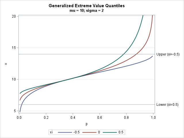
Because the quantile functions are the inverse of the corresponding CDF functions, there is no new information in this plot. Each quantile graph is obtained by rotating the corresponding CDF graphs by 90 degrees and restricting the domain of the CDF function to ensure it is a one-to-one (strictly monotone) function.

You can use the RAND_GEV function to generate random variates from the GEV distribution. The following DATA step generates a random sample of size 1,000 for each ξ value. The SGPANEL procedure is used to visualize the distribution of the samples.

data Rand_Test;
call streaminit(1234);
mu = &mu;
sigma = &sigma;
N = 1000;
do xi = -0.5, 0, 0.5;
do i  = 1 to N;
   x = Rand_GEV(mu, sigma, xi);
   output;
end;
end;
run;
 
title "Generalized Extreme Value Random Variates";
title2 "mu = &mu; sigma = &sigma";
proc sgpanel data=Rand_Test;
   where x < 40;                /* truncate the extreme observations */
   panelby xi / columns=1;
   histogram x;
run;

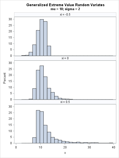
To improve the visualization, I've truncated extreme values of the sample for ξ = 0.5.

Summary

This article shows how to implement four essential functions for working with the generalized extreme value distribution in SAS. The article uses PROC FCMP to define functions that evaluate the CDF, PDF, and quantiles of a GEV distribution, as well as to generate random variates. The formulas for the functions are given in Wikipedia and other online sources. You can store the definitions in a temporary library, as I have done here, or in a permanent library. You use the CMPLIB= option to tell the DATA step where to find the function definitions.

You can implement similar functions in PROC IML, as shown in the Appendix.

Appendix: A SAS IML library for the GEV distribution

If you are a SAS IML programmer, you can define the same functions in the IML language. In the following definitions, the X (or p) argument can be a vector. If so, the function returns a vector of corresponding values. The parameters mu, sigma, and xi are assumed to be scalar values.

/* implement GEV functions in PROC IML */
proc iml;
start CDF_GEV(x, mu, sigma, xi);
   if sigma <= 0 then return( j(nrow(x),ncol(x),.) );
   /* support for x depends on mu - sigma/xi, so support for z depends on -1/xi */
   z = (x-mu)/sigma;
   if xi=0 then                            
      CDF = exp(-exp(-z));                 
   else if xi > 0 then do;
      CDF = j(nrow(x),ncol(x),0);
	  idx = loc(z > -1/xi);
      if ncol(idx)>0 then 
         CDF[idx] = exp(-(1 + xi*z[idx])##(-1/xi));
   end;
   else do; /* xi < 0 */
      CDF = j(nrow(x),ncol(x),1);
	  idx = loc(z < -1/xi);
      if ncol(idx)>0 then 
         CDF[idx] = exp(-(1 + xi*z[idx])##(-1/xi));
   end;
   return (CDF);
finish;
 
start PDF_GEV(x, mu, sigma, xi);
   if sigma <= 0 then return( j(nrow(x),ncol(x),.) );
   z = (x-mu)/sigma;
   if xi=0 then do;
      t = exp(-z);
      PDF = t##(xi+1) # exp(-t) / sigma;
      end;
   else if xi > 0 then do;
      PDF = j(nrow(x),ncol(x),0);
	  idx = loc(z > -1/xi);
      if ncol(idx)>0 then do;
         t = (1 + xi*z[idx])##(-1/xi);
         PDF[idx] = t##(xi+1) # exp(-t) / sigma;
         end;
   end;
   else do; /* xi < 0 */
      PDF = j(nrow(x),ncol(x),0);
	  idx = loc(z < -1/xi);
      if ncol(idx)>0 then do;
         t = (1 + xi*z[idx])##(-1/xi);
         PDF[idx] = t##(xi+1) # exp(-t) / sigma;
         end;
   end;
   return (PDF);
finish;
 
start Quantile_GEV(p, mu, sigma, xi);
   if sigma <= 0 then return( j(nrow(x),ncol(x),.) );
   x = j(nrow(p), ncol(p), .);
   idx = loc(p>0 & p<1);
   if ncol(idx)>0 then do;
	   mLp = -log(p[idx]);
	   if xi=0 then 
	      x[idx] = mu - sigma*log(mLp);
	   else 
	      x[idx] = mu + sigma/xi*(mLp##(-xi) - 1);
	end;
    return (x);
finish;
 
start Rand_GEV(N, mu, sigma, xi);
   p = randfun(N, "Uniform");
   x = Quantile_GEV(p, mu, sigma, xi);
   return (x);
finish;

With these definitions, you can call the CDF, PDF, and quantile functions on a vector of inputs, as follows:

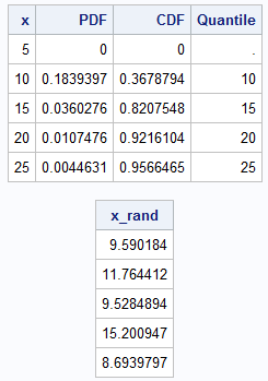
/* show examples for each function call */
mu = &mu;
sigma = &sigma;
xi = 0.5;              /* Frechet distribution */
 
/* test CDF, PDF, and quantile */
x = T( do(5, 25, 5) );
CDF = CDF_GEV(x, mu, sigma, xi);
PDF = PDF_GEV(x, mu, sigma, xi);
Quantile = Quantile_GEV(CDF, mu, sigma, xi);
print x PDF CDF Quantile;
 
/* test random variates */
N = 5;
call streaminit(12345, 1);
x_rand = Rand_GEV(N, mu, sigma, xi);
print x_rand;

Blogs