While researching a topic on effect sizes, I learned about a SAS function that is related to noncentrality parameters. I previously wrote an article about the noncentral t distribution, which is one of several well-known distributions that contains an optional noncentrality parameter. I mentioned that the PDF, CDF, and QUANTILE functions in SAS support an optional noncentrality parameter for the t, chi-square, and F distributions.

However, I did not know until recently that SAS also provides related computational functions that are used for estimating confidence intervals of the noncentral parameter. The functions are named TNONCT, CNONCT, and FNONCT. These functions enable you to estimate confidence intervals for noncentrality parameters.

This article discusses the TNONCT function in SAS, which is used to construct confidence intervals for effect-size statistics that follow a noncentral t distribution. The FNONCT function (for the noncentral F distribution) and the CNONCT function (for the noncentral chi-square distribution) are similar.

Review of the noncentral t distribution

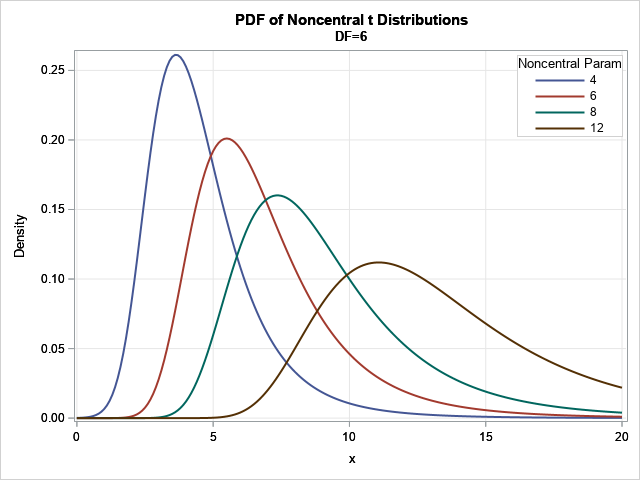
See my previous article for a discussion of the noncentral t distribution. The graph at the right shows noncentral t distributions for four values of the noncentral parameter for a t distribution that has 6 degrees of freedom (DF=6). You can see that the noncentral parameter causes the mode of the distribution to shift. It also causes the distribution to have skewness. When the noncentrality parameter is 0, the distribution is symmetric and the mode is at x=0.

The graphs are drawn by using the PDF function with the optional noncentrality parameter. The SAS documentation calls it 'nc', but I will use the symbol δ. (The symbol λ is also used in the literature.) The CDF and QUANTILE functions also support δ. You can use these functions to find critical points and probabilities for the noncentral t distribution. For example, let α = 0.05 be a left-tail probability. The following SAS DATA step find the critical point, x_c, for the left tail of the t(DF=6, δ=8) distribution.

data Quantile;
alpha = 0.05;   /* probability */
DF = 6;         /* degree-of-freedom parameter */
delta = 8;      /* noncentrality parameter */
x_c = quantile("t", alpha, DF, delta);  /* find 0.05 quantile */
prob =  CDF("t", x_c, DF, delta);       /* check to make sure we get back alpha */
run;
 
proc print noobs; run;

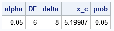
Notice that the CDF function returns the left-tail probability up to a value of x whereas the QUANTILE function solves the inverse problem and returns the x value for which CDF("t", x, DF, δ) = α. These functions require that you know the parameters for the noncentral t distribution, which are DF and δ. If you want the critical point for the right-tail probability, you can use 1 – α for the probability parameter.

What value of the noncentrality parameter has a given critical value?

The QUANTILE function solves an inverse problem: given DF, δ, and α, find the value of x for which CDF("t", x, DF, δ) = α. The TNONCT function also solves an inverse problem, but it solves for δ instead of x. In other words, it assumes that you know x, DF, and the α probability, and you want to find the noncentrality parameter.

For example, suppose DF=6, α=0.05, and x=5. What is the value of the noncentrality parameter, δ, for which the distribution t(DF, δ) has a left-tail probability of α at the critical point x=5?

The noncentrality parameter shifts the density curve and also changes its shape. Notice in the previous example that the critical value for the t(DF=6,delta=8) curve was x = 5.2. If we choose different value of the noncentrality parameter, delta, we expect the critical value to change as well. Intuitively, the graph suggests if we decrease the value of δ (make it less than 8), the critical point of the distribution should also decrease from 5.2. We just need to figure out how much smaller to make δ.

You can call the QUANTILE function with a sequence of δ values to visualize how the critical value for x depends on the noncentrality parameter:

data NoncentralParam;
label delta='Noncentrality Parameter' x_c='Critical Value for alpha=0.05';
alpha = 0.05;   /* probability */
DF = 6;         /* degree-of-freedom parameter */
do delta = 4 to 12 by 0.1;
   x_c = quantile("t", alpha, DF, delta);  /* for each delta value, find critical value */
   output;
end;
run;
 
title "Critical Value for alpha=0.05 versus Noncentrality Parameter in t Distribution";
proc sgplot data=NoncentralParam;
   series  x=delta y=x_c;
   xaxis grid values=(4 to 12);
   yaxis grid values=(2 to 8);
run;

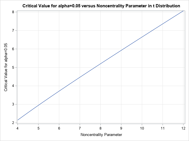
The graph shows that the relationship between δ and the critical value is monotonic. From the graph, you can estimate that the critical point is x=5 when the noncentrality parameter is approximately 7.7.

The TNONCT function enables you to find the exact value of δ by using a single function call. If delta = TNONCT(x, DF, alpha), then delta is the value of the noncentrality parameter for which CDF("t", x, DF, delta) = alpha. The following call to the TNONCT function finds the value of δ when x=5:

data tnonct;
alpha = 0.05;   /* probability */
DF = 6;         /* degree-of-freedom parameter */
x_c = 5;        /* critical value */
delta_U = tnonct(x_c, DF, alpha);
delta_L = tnonct(x_c, DF, 1-alpha);
run;
 
proc print noobs; run;

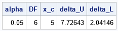
The table shows that when δ = δ_U = 7.726, the distribution t(DF=6, δ_U) has a left-tail probability of α at the critical point x=5. I also computed the noncentrality parameter for which the left-tail probability is 1 – α, or, equivalently, for which the right-tail probability is α. The distribution with δ = δ_L = 2.041 has that property. The following graph visualizes both distributions. I have shaded the left tail when δ = 7.726 and shaded the right tail when δ = 2.041.

Why should you care?

Some statistics follow a noncentral t distribution, and you can use the TNONCT function to estimate confidence intervals for the underlying parameters. I don't have space in this article to show an example, but δ_L is used to construct a lower limit for a CI and δ_U is used to construct an upper limit.

Summary

This article shows how to use the TNONCT function in SAS to find the value of the noncentrality parameter (δ) for the t distribution such that t(DF, δ) has a left-tail probability of α at a specified location for x. That is, given values for DF, α and x, find the value of δ for which CDF("t", x, DF, δ) = α. The TNONCT function is used to estimate confidence intervals for some effect-size statistics.

Similar functions exist for the F and chi-square distributions. The FNONCT function solves for the noncentral parameter in an F distribution; the CNONCT function solves for the noncentral parameter in a chi-square distribution.