A previous article discusses Cohen's d statistic and how to compute it in SAS. For a two-sample independent design, Cohen's d estimates the standardized mean difference (SMD). Because Cohen's d is a biased statistic, the previous article also computes Hedges' g, which is an unbiased estimate of the SMD. Lastly, the article discusses how to estimate the standard error of the statistic. Today's article extends the analysis by showing how to compute a confidence interval (CI) for Cohen's d (and Hedges' g) in SAS. The primary reference for this blog post is Goulet-Pelletiera and Cousineau (2018), which is an excellent resource that I highly recommend.
Confidence intervals from the noncentral t distribution
The (central) t distribution is a well-known symmetric distribution that is centered at 0. For some elementary statistics (such as a mean), confidence intervals are of the form p ± tc*SE, where p is a point estimate, SE is a standard error, and tc is a critical value for the symmetric t distribution. The critical value is chosen to provide a "coverage factor" such as a 90% or a 95% CI. You can form a CI of this form by using p=d (or p=g for Hedges' statistic) and the standard error (SE) that I showed in the previous article.
You can generalize the t distribution by adding a noncentrality parameter, which causes the mode of the distribution to shift. It also causes the distribution to have skewness. For more details, read my previous article about the noncentral t distribution.
It turns out that the confidence interval for Cohen's d is not symmetric. Goulet-Pelletiera and Cousineau (2018) show how to use a noncentral t distribution to obtain a confidence interval. They state emphatically, "the noncentral CI is without a doubt the most reliable method especially when n is smaller than 20" (p.251). They repeat this assertion in the conclusions: "the noncentral method is superior to the central method" (p. 255).
To use a noncentral t distribution, you must have an estimate for
the noncentrality parameter. For the two-sample independent design,
the noncentrality parameter is estimated by
\(
\lambda = \delta / \sqrt{2/\tilde{n}}
\)
where \(\tilde{n} = 2 n_1 n_2/(n_1+n_2)\) is the harmonic mean of the group sizes, n1 and n2.
Here, δ is an estimate of the SMD, such as either Cohen's d or Hedges' g.
This leads to the following SAS statements, which you can add to the DATA step in the previous article:
lambda = delta / sqrt(w); /* noncentrality parameter for t distribution (2 indep groups) */ alpha = 0.05; /* for a (1-alpha)*100% CI */ t_lower = quantile("t", alpha/2, df, lambda); /* noncentral t, alpha/2 quantile */ t_upper = quantile("t", 1-alpha/2, df, lambda); /* noncentral t, 1-alpha/2 quantile */ /* transform CI for t into CI for delta. Note: This actually reduces to t*sqrt(w) */ delta_lower = t_lower / (lambda/delta); /* LCL for effect size, delta */ delta_upper = t_upper / (lambda/delta); /* UCL for effect size, delta */ |
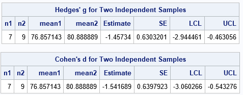
You can download the complete SAS program that uses PROC TTEST and the DATA step to compute Cohen's d and Hedges' g statistic, along with estimates of the standard error and confidence intervals. If you run the example from the previous article and include a 95% confidence interval, you get the following result:
Because the 95% CI does not include 0, you can conclude that (with 95% confidence) the SMD is not 0.
Notice that the CI is not centered about the estimate. The width of the left subinterval (from the lower limit to the estimate) is a little less than 1.5 whereas the width of the right subinterval (from the estimate to the upper limit) is about 1.0.
For completeness, I've also written a SAS IML program that encapsulates the computations into callable functions. This is shown in the Appendix, or you can download the SAS IML program from GitHub.
Summary
This article completes the task of showing how to compute Cohen's d and Hedges' g statistic in SAS when data are from a design that compares the means of two independent samples. These statistics estimate the standardized mean difference between the groups. The CI computations assume that each subpopulation is normally distributed with the same variance. This article uses the computations outlined in Goulet-Pelletier & Cousineau (2018), who emphasize three things:
- "Hedges’ g should always be preferred over Cohen’s d" (G-P & C, p. 245).
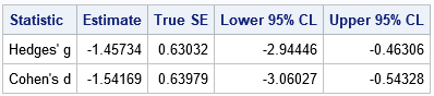
- The best estimate of SE is called the "True SE" in G-P & C.
- "The noncentral CI is without a doubt the most reliable method especially when n is smaller than 20" (G-P & C, p. 251). In fact, CIs obtained from noncentral t distribution are exact for Hedges' g.
The Goulet-Pelletier & Cousineau (2018) article contains a discussion of other designs, such as one-sample tests and tests for paired data. You can modify my program to compute these other statistics.
Appendix: SAS IML program for computing Cohen's d and confidence intervals
/* Use PROC IML to implement the formulas in Goulet-Pelletier & Cousineau (2018) for Cohen's d and Hedges' g */ /* data from PROC TTEST documentation: Golf scores for students in a physical education class */ data scores; input Gender $ Score @@; datalines; f 75 f 76 f 80 f 77 f 80 f 77 f 73 m 82 m 80 m 85 m 81 m 78 m 83 m 82 m 76 m 81 ; /* computation of Cohen's d and Hedges' g in SAS IML. Helper Functions: run Indep2SampleStats(...) : get descriptive statistics mean1, mean2, n1, n2, df, pooled std dev delta = EffectSize(...) : estimate effect size by using Cohen's d or Hedges' g SE = EffectSize_SE(delta,...) : estimate standard error of estimate of effect size CI = EffectSize_SE(delta,...) : estimate confidence interval for effect size */ proc iml; /* get descriptive statistics mean1, mean2, n1, n2, df, pooled std dev */ start Indep2SampleStats(m1, m2, n1, n2, df, s_p, /* output stats */ Group, Y); /* input stats */ u = unique(Group); x1 = Y[ loc(Group=u[1]) ]; /* reference group */ n1 = countn(x1); m1 = mean(x1); s1 = std(x1); x2 = Y[ loc(Group=u[2]) ]; /* comparison group */ n2 = countn(x2); m2 = mean(x2); s2 = std(x2); df = n1 + n2 - 2; s_p = sqrt( ((n1-1)*s1##2 + (n2-1)*s2##2) / df ); /* pooled SD */ finish; /* estimate the effect size. Return Cohen's d if STAT="D", otherwise return Hedges' g */ start EffectSize(m1, m2, n1, n2, s_p, stat="G"); /* input statistics */ d = (m1 - m2) / s_p; /* Cohen's d, which is a biased estimator */ if upcase(stat)="D" then return( d ); /* J is Hedge's correction factor. See Cousineau & Goulet-Pelletier (2020, p. 244) */ df = n1 + n2 - 2; /* degrees of freedom */ J = exp( lgamma(df/2) - lgamma((df-1)/2) - log(sqrt(df/2)) ); g = J * d; /* Hedge's g, which is an unbiased estimator */ return( g ); finish; /* estimate standard error of estimate of effect size */ start EffectSize_SE(delta, n1, n2); /* the harmonic mean of n1 and n2 is 2*n1*n2/(n1+n2) */ w = 2/harmean(n1//n2); /* 2/H(n1,n2) = (n1+n2)/(n1*n2) */ df = n1 + n2 - 2; /* degrees of freedom */ J = exp( lgamma(df/2) - lgamma((df-1)/2) - log(sqrt(df/2)) ); /* The best estimate of standard error is the "true formula" */ var = df/(df-2) * (w + delta**2) - (delta/J)**2; return( sqrt(var) ); finish; /* estimate confidence interval for effect size */ start EffectSize_CI(delta, n1, n2, alpha=0.05); /* the harmonic mean of n1 and n2 is 2*n1*n2/(n1+n2) */ w = 2/harmean(n1//n2); /* 2/H(n1,n2) = (n1+n2)/(n1*n2) */ df = n1 + n2 - 2; /* degrees of freedom */ /* CIs obtained from noncentral t distribution; this is exact for Hedges' g */ lambda = delta / sqrt(w); /* noncentrality parameter for t distribution (2 indep groups) */ t_lower = quantile("t", alpha/2, df, lambda); /* alpha/2 quantile */ t_upper = quantile("t", 1-alpha/2, df, lambda); /* 1-alpha/2 quantile */ /* transform CI for t into CI for delta */ delta_lower = t_lower / (lambda/delta); delta_upper = t_upper / (lambda/delta); return( delta_lower || delta_upper ); finish; /* test the functions on the golf score data */ DSName = "Scores"; ClassName = "Gender"; YName = "Score"; use (DSName); read all var ClassName into Group; read all var YName into Y; close; run Indep2SampleStats(m1, m2, n1, n2, df, s_p, /* output stats */ Group, Y); /* input stats */ *print n1 n2 m1 m2 df s_p; /* Hedges' g statistic */ g = EffectSize(m1, m2, n1, n2, s_p); /* default is Hedges' g */ g_SE = EffectSize_SE(g, n1, n2); g_CI = EffectSize_CI(g, n1, n2); g_results = n1 || n2 || m1 || m2 || g || g_SE || g_CI; lbl = {'n1' 'n2' 'mean1' 'mean2' 'Estimate' 'SE' 'LCL' 'UCL'}; print g_results[c=lbl L="Hedges' g for Two Independent Samples"]; /* Cohen's d statistic */ d = EffectSize(m1, m2, n1, n2, s_p, "D"); d_SE = EffectSize_SE(d, n1, n2); d_CI = EffectSize_CI(d, n1, n2); d_results = n1 || n2 || m1 || m2 || d || d_SE || d_CI; print d_results[c=lbl L="Cohen's d for Two Independent Samples"]; |