The noncentral t distribution in SAS

The noncentral t distribution is a probability distribution that is used in power analysis and hypothesis testing. The distribution generalizes the Student t distribution by adding a noncentrality parameter, δ. When δ=0, the noncentral t distribution is the usual (central) t distribution, which is a symmetric distribution. When δ > 0, the noncentral t distribution is positively skewed; for δ < 0, the noncentral t distribution is negatively skewed. Thus, you can think of the noncentral t distribution as a skewed cousin of the t distribution.

SAS software supports the noncentrality parameter in the PDF, CDF, and QUANTILE functions. This article shows how to use these functions for the noncentral t distribution. The RAND function in SAS does not directly support the noncentrality parameter, but you can use the definition of a random noncentral t variable to generate random variates.

Visualize the noncentral t distribution

The classic Student t distribution contains a degree-of-freedom parameter, ν. (That's the Greek letter "nu," which looks like a lowercase "v" in some fonts.) For small values of ν, the t distribution has heavy tails. For larger values of ν, the t distribution resembles the normal distribution. The noncentral t distribution uses the same degree-of-freedom parameter.

The noncentral t distribution also supports a noncentrality parameter, δ. The simplest way to visualize the effect of δ is to look at its probability density function (PDF) for several values of δ. The support of the PDF is all real numbers, but most of the probability is close to x = δ. You can use the PDF function in SAS to compute the PDF for various values of the noncentrality parameter. The fourth parameter for the PDF("t",...) call is the noncentrality value. It is optional and defaults to 0 if not specified.

The following visualization shows the density functions for positive values of δ and positive values of x. In the computer programs, I use DF for the ν parameter and NC for the δ parameter.

/* use the PDF function to visualize the noncentral t distribution */
%let DF = 6;
data ncTPDFSeq;
df = &DF;                        /* degree-of-freedom parameter, nu */
do nc = 4, 6, 8, 12;             /* noncentrality parameter, delta */
   do x = 0 to 20 by 0.1;        /* most of the density is near x=delta */
      PDF = pdf("t", x, df, nc);
      output;
   end;
end;
label PDF="Density";
run;
 
title "PDF of Noncentral t Distributions";
title2 "DF=&DF";
proc sgplot data=ncTPDFSeq;
   series x=x y=PDF / group=nc lineattrs=(thickness=2);
   keylegend / location=inside across=1 title="Noncentral Param" opaque;
   xaxis grid; yaxis grid;
run;

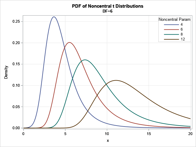
The graph shows the density functions for δ = 4, 6, 8, and 12 for a distribution that has ν=6 degrees of freedom. You can see that the modes of the distributions are close to (but a little less than) δ when δ > 0. For negative values of δ, the functions are reflected across x=0. That is, if f(x; ν, δ) is the pdf of the noncentral t distribution with parameter δ, then f(-x; ν, -δ) = f(x; ν, δ).

The CDF and quantile function of the noncentral t distribution

If you change the PDF call to a CDF call, you obtain a visualization of the cumulative distribution function for various values of the noncentrality parameter, δ.

The quantile function is important in hypothesis testing. The following DATA step finds the quantile that corresponds to an upper-tail probability of 0.05. This would be a critical value in a one-sided hypothesis test where the test statistic is distributed according to a noncentral t distribution.

%let NC = 4;
data CritVal;
do alpha = 0.1, 0.05, 0.01;
   tCritUpper = quantile("T", 1-alpha, &DF, &NC);
   output;
end;
run;
 
proc print data=CritVal nobs; run;

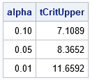
The graph shows the critical value of a noncentral t statistic for a one-sided hypothesis test at the α significance level for α=0.1, 0.05, and 0.01. A test statistic that is larger than the critical value would lead you to reject the null hypothesis at the given significance level.

Random variates from the noncentral t distribution

Although the RAND function in SAS does not support a noncentrality parameter for the t distribution, it is simple to generate random variates. By definition, a noncentral t random variable, T_{ν δ} is the ratio of a standard normal variate with mean δ and a scaled chi-distributed variable. If Z ~ N(δ,1) is a normal random variable and V ~ χ²(ν) is a chi-squared random variable with ν degrees of freedom, then the ratio T_{ν δ} = Z / sqrt(V / ν) is a random variable from a noncentral t distribution.

/* Rand("t",df) does not support a noncentrality parameter. Use the definition instead. */
data ncT;
df = &DF;
nc = &NC;
call streaminit(12345);
do i = 1 to 10000;
   z = rand("Normal", nc);   /* Z ~ N(nc, 1)    */
   v = rand("chisq", df);    /* V ~ ChiSq(df)   */
   t = z / sqrt(v/df);       /* T ~ NCT(df, nc) */
   output;
end;
keep t;
run;
 
title "Random Sample from Noncentral t distribution";
title2 "DF=&DF; nc=&NC";
proc sgplot data=ncT noautolegend;
   histogram t;
   density t / type=kernel;
   xaxis max=20;
run;

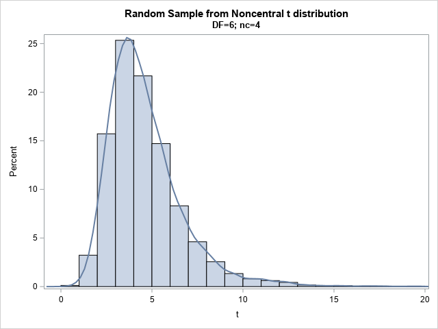
The graph shows a histogram for 10,000 random variates overlaid with a kernel density estimate. The density is very similar to the earlier graph that showed the PDF for the noncentral t distribution with ν=6 degrees of freedom and δ=4.

Summary

The noncentral t distribution is a probability distribution that is used in power analysis and hypothesis testing. You can this of the noncentral t distribution as a skewed t distribution. SAS software supports the noncentral t distribution by using an optional argument in the PDF, CDF, and QUANTILE functions. You can generate random variates by using the definition of a random variable, which is a ratio of a normal variate and a scaled chi-distributed variable.

Blogs