Implement a SMOTE simulation algorithm in SAS

A recent article describes the main features of simulation by using the Synthetic Minority Over-sampling Technique (SMOTE). SMOTE was created to oversample from a set of rare events prior to running a machine learning classification algorithm. However, at its heart, the SMOTE algorithm (Chawla et al., 2002) provides a way to simulate new synthetic data from real data.

The Visual Data Mining and Machine Learning (VDMML) license in SAS Viya supports the smote action set, which contains the smoteSample action. In addition to the documentation examples, there is a GitHub site that describes how to use the action to generate synthetic data. The smoteSample action can simulate from data that contains both continuous and nominal variables.

When I want to understand an algorithm, I find it instructive to implement it in SAS from basic principles. This article uses the SAS IML language to implement a simple SMOTE algorithm. It requires that all data variables are continuous. For a version of SMOTE that uses the DATA step and the MODECLUS procedure, see the Appendix of Boardman, Biron, and Rimbey (2018), which includes a SAS program that uses the DATA step and the MODECLUS procedure to implement a SMOTE algorithm for continuous data. The program is hard-coded for a specific data set, but it could be modified for other data.

The SMOTE algorithm

The SMOTE algorithm generates a new synthetic data point by using linear interpolation among the data values. If P and Q are two data points, SMOTE generates a new synthetic observation by placing a random point on the line segment connecting P and Q. In equation form, the new synthetic observation is Z = P + u*(Q-P), where u ~ U(0,1) is a random uniform variate.

The basic SMOTE algorithm uses three input parameters:

X: An N x d data matrix. The rows of X are the d-dimensional points used to generate the synthetic data. We name the points by their row number: X1, X2, ..., XN.
k: the number of nearest neighbors, where 1 ≤ k ≤ N. For each X_i, compute the k points that are closest to X_i in the Euclidean distance. For efficiency, compute the nearest neighbors once and remember that information.
T: the number of new synthetic data points that you want to generate.

The simple SMOTE algorithm generates synthetic data by doing the following:

Choose T rows uniformly at random (with replacement) from the set 1:N. These rows of the X matrix correspond to the "P" points, which define one end of a line segment.
For each point, P, choose a point uniformly at random from among the k neighbors nearest to P. These represent the "Q" points, which define the other end of a line segment.
For each pair, P and Q, generate a uniform random variate in the interval (0,1). The new synthetic data point is Z = P + u*(Q-P).

Example data for the SMOTE simulation

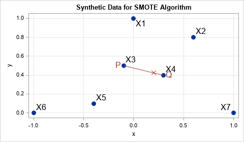
Let's run a SMOTE simulation on a small data set that contains seven observations and two variables. The following DATA step defines the data and creates a scatter plot of the seven observations:

data SmallData;
input ID $ x y;
datalines;
X1  0   1
X2  0.6 0.8
X3 -0.1 0.5
X4  0.3 0.4
X5 -0.4 0.1
X6 -1   0 
X7  1   0
;

A scatter plot of the data is shown in the previous section. The scatter plot displays a random point (P) and a random nearest neighbor (Q) to that point. A synthetic data point is generated along the line segment connecting P and Q.

Implement SAS IML functions for the SMOTE algorithm

By using the SAS IML language, you can implement the simple SMOTE algorithm by writing three user-defined modules:

NearestNbr: This subroutine is described in a previous article about nearest-neighbor computations. The input parameters are the data matrix, X, and the number of nearest neighbors, k. The module outputs two arguments. The first output argument is an N x k matrix of row numbers, NN. The integer NN[i,j] contains the row numbers (in X) of the j_th closest neighbor to the observation X[i,]. The second output argument (DIST) is the corresponding matrix of distances between X[i,] and its nearest neighbors. We do not need to use the second output argument for SMOTE. Note: The subroutine computes the N x k matrix of pairwise distances between observations. This puts a limit on the size of the data that can be used. I suggest N ≤ 16000. For larger data sets, rewrite the subroutine or consider using the smoteSample action in Viya.
RandRowsAndNbrs: This function performs the random selection of the P and Q data points. The input arguments are T and NN. T is the number of desired synthetic data points. NN is the N x k integer matrix of nearest neighbor information that was returned by the NearestNbr routine. The function outputs a T x 2 integer matrix, R. The first column of R contains random rows of X. The second column contains rows for a nearest neighbor.
SMOTESimContin: This function implements the simple SMOTE algorithm by calling the previous two routines and then performing the random interpolation between each P and Q point. The inputs to the function are the data matrix (X), the number of synthetic points to generate (T), and the number of nearest neighbors to use (k). The function returns a T x d matrix where each row is a synthetic data point.

You can download the PROC IML program that defines the functions. Before you can use the modules, you must run the program in module definition file, which stores the modules. Do that now, if you want to run the programs in this article.

Testing the IML modules

In practice, the only module you need to call is the SMOTESimContin function, which returns the synthetic data. However, for the purpose of understanding the algorithm, let's look at the other two helper functions to see how they work.

The following PROC IML statements load the helper modules, read the data into a matrix, X, and then call the NearestNbr module with k=3 to compute the nearest-neighbor matrix.

/* example: How to call the helper routines for SMOTE simulation */
proc iml;
load module=(NearestNbr RandRowsAndNbrs SMOTESimContin);  /* load the helper functions */
use SmallData;                                            /* read the example data */
   read all var {'x' 'y'} into X;
close;
 
k = 3;                                                    /* number of nearest neighbors */
run NearestNbr(NN, dist, X, k);                           /* get the nearest-neighbor matrix */
print NN[r=('X1':'X7')];

You can read more about the nearest-neighbor computations, but the output matrix tells you the three nearest neighbors for each row of X. The first row of NN tells you that the nearest neighbors to X1 are X3, X2, and X4. The second row of NN tells you that the nearest neighbors to X2 are X4, X1, and X3. Notice that the NN matrix contains row numbers. If you want the coordinates of the points, you must index into the X matrix. For example, the coordinates of the nearest points to X1 are given by X[3,], X[2,], and X[4,].

Although it is not required for this example, note that the Euclidean distance is used to compute the nearest neighbors. If all variables are not measured in the same units, it is best to standardize the variables before passing them to the NearestNbr subroutine. Failure to standardize the variables will affect the quality of the synthetic data. Of course, after generating the synthetic data, you need to use the inverse transformation to convert it back to the scale of the original variables.

The next step of the SMOTE simulation algorithm is to generate random points in X and, for each random point, a random nearest neighbor. This is done automatically by calling the RandRowsAndNbrs function. You don't need to know the details, but the RandRowsAndNbrs function samples with replacement from the set {1,2,...,N} to obtain a random row of X to use for P. It then randomly selects an integer in the set {1,2,...,k} and looks up the nearest neighbor of P by using the NN matrix. The following snippet calls the RandRowsAndNbrs function and requests 20 random (P,Q) pairs.

call randseed(321);
T = 20;
R = RandRowsAndNbrs(T, NN);
print R[c={"P" "Q"}];

The full output contains T=20 rows, but only a few are shown. The first row indicates that the first point is X3 and that X4 is randomly chosen from among its three nearest neighbors. The second row indicates that the second point is X5 and that X3 is randomly chosen from among its three nearest neighbors. In general, R[i,1] is the i_th value of P and R[i,2] is the i_th value of Q.

Run the SMOTE simulation on a small example

As mentioned earlier, the only function you really need to call is the SMOTESimContin function. The following program restarts PROC IML, loads the data and the modules, and generates T=20 synthetic data points by using the SMOTE simulation method:

proc iml;
load module=(NearestNbr RandRowsAndNbrs SMOTESimContin);  /* load the helper functions */
use SmallData;                                            /* read the example data */
   read all var {'x' 'y'} into X;
close;
 
call randseed(321);
k = 3;                                                    /* number of nearest neighbors */
T = 20;                                                   /* number of synthetic data points */
X_synth = SMOTESimContin(X, T, k);
print X_synth[c={'sx' 'sy'}];

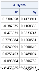
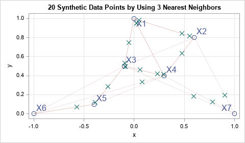
The output shows the (x,y) coordinates of the first few synthetic data points. Each of the points lies on a line segment between two original data points. You can overlay the synthetic data on a scatter plot of the original data. For clarity, I also added line segments between each point and its three nearest neighbors.

Run the SMOTE simulation on Fisher's iris data

The previous data are two-dimensional and very small. Let's run the simulation algorithm on a larger data set and compare the descriptive statistics of the real data and the simulated data. The following data set extracts 50 observations where Species='Versicolor' in Fisher's iris data. This is four-dimensional data. The SAS IML code is almost identical, except this example simulates T=100 new synthetic values:

/* extract one species of iris data */
data Versicolor;
set sashelp.iris(where=(species='Versicolor'));
attrib _all_ label=' ';
run;
 
proc iml;
load module=(NearestNbr RandRowsAndNbrs SMOTESimContin);
use Versicolor;
read all var _NUM_ into X[c=varNames];
close;
 
call randseed(321);
k = 5;
T = 100;
X_synth = SMOTESimContin(X, T, k);
 
create synthetic from X_synth[c=varNames];
append from X_synth;
close;
QUIT;
 
/* compare descriptive statistics for the original and synthetic data */
title "50 Iris Data Points (Species='Versicolor')";
proc corr data=Versicolor noprob cov plots=matrix(histogram);
var _numeric_;
run;
 
title "100 Synthetic Data Points by Using 5 Nearest Neighbors";
proc corr data=synth_iris noprob cov plots=matrix(histogram);
var _numeric_;
run;

The following output (from PROC CORR) shows the simple descriptive statistics and the correlations between variables in the original data and in the synthetic sample:

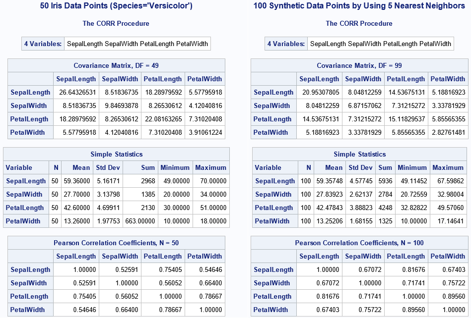
The statistics for the real data are shown on the left; the statistics for the synthetic data are on the right. There are some important differences between the statistics for the real data and for the synthetic data. For the "Covariance Matrix" table, all variances and covariances for the synthetic data are smaller in magnitude than for the real data. The variances (on the matrix diagonal) are shrunk towards 0 by more than the covariances, which means that the correlations in the "Pearson Correlation Table" are systematically stronger for the synthetic data as compared to the real data.

For the univariate statistics in the "Simple Statistics" table:

Mean column: The means of the synthetic variables are close to the means of the original data. This is good!
Std Dev column: The standard deviations of the synthetic variables are systematically smaller than the standard deviations of the original data.
Minimum and Maximum columns: The ranges of the synthetic variables are systematically smaller than the ranges of the original data. This is obvious by understanding the SMOTE construction.

The statements about the descriptive statistics agree with my intuition, which is based on the geometry of the algorithm. For a continuous variable, you should expect the ranges of the synthetic variables to be systematically smaller than the ranges of the original data.

It is harder to make general statements about the standard deviation because the mean and standard deviation are not robust statistics and because the simulated data is random. For tame data (for example, normal data), I would expect the standard deviation of the synthetic data to be smaller. For data with extreme outliers, it is not clear what might happen. For some random samples, the outliers might not be selected, which can radically change the mean and standard deviation statistics. For other samples, the outliers might be chosen multiple times, which could inflate the standard deviation.

It is best not to generalize from a few examples. Consequently, I do not claim that the statements about covariances and correlation generalize to other data sets. I have seen an example where the correlations among the synthetic variables were smaller than for the real variables.

I did a quick literature search to see whether someone has performed a comprehensive study of the statistical properties of the synthetic data from SMOTE. I didn't find a paper that addresses this question directly. Figure 5 in Houssdou et al. (2022) show a similar result, but the authors did not comment on it. Post a comment if you can provide a reference for a peer-reviewed study that explores the statistical properties of the SMOTE synthetic data and how they compare to the properties of the real data.

Summary

This article shows how to implement a simple SMOTE simulation algorithm in SAS by using the SAS IML language. The simulation is valid for continuous numerical variables. You can download the file that defines the IML modules. You can also download the file that contains all programs for this article (and more!).

In addition to running the SMOTE simulation on a small example, I also ran the data on larger examples. The example that uses Fisher's Iris data shows that the synthetic data from the simple SMOTE algorithm can exhibit systematic bias. Namely, the variance of the synthetic variables can be smaller than for the original data. For this example, the synthetic variables had smaller variance-covariance and larger correlations. Of course, this was for a single random sample, so we shouldn't over-generalize. A more systematic simulation study is warranted.

I ran other examples (not shown here) that used data that was not as "tame" as the Iris data. I observed that many (but not all) synthetic variables had a smaller variance than their real counterparts. The covariances and correlations for the synthetic variables were sometimes larger and sometimes smaller.

Blogs