The Synthetic Minority Over-sampling Technique (SMOTE) was created to address class-imbalance problems in machine learning algorithms. The idea is to oversample from the rare events prior to running a machine learning classification algorithm. However, at its heart, the SMOTE algorithm (Chawla et al., 2002) is essentially a way to simulate new synthetic data from real data.

This article looks at the SMOTE algorithm with a focus on the geometry of the simulation of synthetic data. Because I am interested in simulation (not classification), when I say, "the data," I always mean the data from which we are simulating. Traditionally, this is the minority class (rare events).

A later article will demonstrate how you can implement a simple SMOTE algorithm in SAS.

The basic SMOTE algorithm

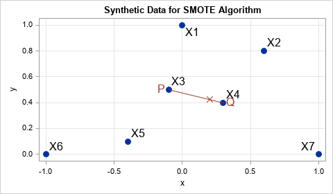
There have been many papers that describe variations on the SMOTE algorithm, but the basic idea is to use linear interpolation between data points. If you are given two real observations, P and Q, you can generate a new synthetic observation by placing a random point on the line segment connecting P and Q. In equation form, the new synthetic observation is Z = P + u*(Q-P), where u ~ U(0,1) is a random uniform variate.

An example is shown in the graph to the right. The points X1, X2, ..., X7 are the data points. The point X3 is selected at random to be P. From among the data points close to P, the point X4 is selected at random to be Q. Then a synthetic point (marked with an X) is chosen at random along the line segment from P to Q.

There are various ways to select P and Q. In this article, P will be selected by randomly sampling (with replacement) from the original set of observations. After selecting P, you look at the k nearest neighbors of P, where k is a parameter in the SMOTE algorithm. (The original paper uses k=5.) The point Q is chosen from among those nearest neighbors. In this article, Q will be chosen uniformly at random from among the k nearest neighbors.

A SMOTE algorithm

As described above, the SMOTE algorithm uses linear interpolation between nearest neighbors to simulate synthetic data. For simplicity, I assume that all variables are continuous.

1. Input an N x d data matrix, X. The rows of X are the d-dimensional points used to generate the synthetic data. We will name the points by their row number: X1, X2, ..., XN.
2. Specify k, the number of nearest neighbors, where 1 ≤ k ≤ N. For each X_i, compute the k points that are closest to X_i in the Euclidean distance. For efficiency, you can compute the nearest neighbors once and remember that information.
3. Specify T, the number of new synthetic data points that you want to generate.
4. Choose T rows uniformly at random (with replacement) from the set 1:N. These represent the "P" points, which define one end of a line segment.
5. For each point, P, choose a point uniformly at random from among the k neighbors nearest to P. These represent the "Q" points, which define the other end of a line segment.
6. For each pair, P and Q, generate a uniform random variate in the interval (0,1). The new synthetic data point is Z = P + u*(Q-P).

The geometry of SMOTE

A key geometric fact is that SMOTE generates synthetic data only on line segments connecting the original data. The synthetic data look like "spokes" emanating from a hub. In other words, the probability density for the synthetic data is supported only on one-dimensional line segments. This is different from other methods for generating multivariate data. For example, the multivariate normal distribution has a density function whose support is d-dimensional. The random variates can appear anywhere in a d-dimensional region.

The line segments in the following graph are the possible locations of synthetic SMOTE data that are generated from seven points in 2-D. For this example, k=3. The synthetic data must appear on the line segments that connect observations to their three nearest neighbors.

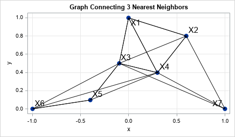
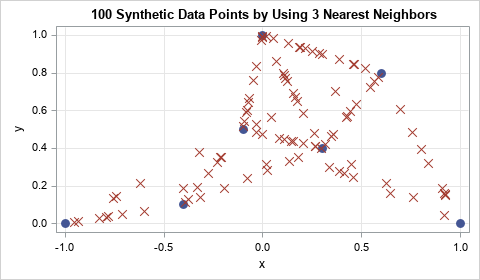
2-D Synthetic data from SMOTE

The graph below shows 100 synthetic data points that are generated from the seven original data points when k=3. The original data are represented by seven circular markers. The 'X' markers represent the synthetic data. I have removed the line segments, but you can clearly see that the synthetic data appear along the line segments.

Synthetic data for 4-D iris data

Up to now, the examples have been two-dimensional, but the SMOTE simulation method works for higher-dimensional data. The famous Fisher's Iris data set (SASHELP.IRIS in SAS) has 50 observations that belong to the class Species="Versicolor". Each observation records the length and height of the petals and sepals of a flower. I ran the SMOTE algorithm with k=5 nearest neighbors to generate 100 synthetic data values from the Versicolor iris data measurements. The following output (from PROC CORR) shows the simple descriptive statistics and the correlations between variables in the original data and in the synthetic sample:

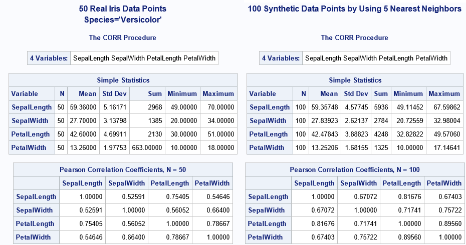
The statistics for the real data are shown on the left; the statistics for the synthetic data are on the right. Although the statistics are generally close, there are a few important differences in the statistics, which I will discuss in a subsequent article.

Summary

SMOTE was created to address class-imbalance problems in machine learning algorithms. But some people use the SMOTE algorithm to simulate new synthetic data. This article provides an overview of simulation by using the SMOTE algorithm. I did not perform a serious study that compares the statistical properties of the real and synthetic properties, but the geometry of the algorithm suggests that the synthetic data will tend to have smaller variances and larger correlations.

Appendix: Additional comments about using the SMOTE algorithm for data simulation

To prevent the article from being too long, I moved two discussion topics into this Appendix: how the scaling of variables affects the SMOTE algorithm and how to choose k, the number of nearest neighbors.

Scaling and standardizing: The Euclidean distance is used to compute the nearest neighbors. When all variables are continuous, this makes intuitive sense. If some variables are not measured in the same units, it is best to standardize the variables. The examples in this article do not require any standardization methods, but in practice the scales of the variables are important because they determine which observations are near one another. If you measure a length in inches, the Euclidean distances between the measurements are smaller than if you measure the length in centimeters. Thus, the SMOTE algorithm depends on the scaling of the data. If you are using the SMOTE algorithm, I encourage you to standardize continuous variables by using a robust measure of scale.

Choosing the number of nearest neighbors: For many data sets, it is not clear how to choose the number of nearest neighbors that are used in SMOTE. Chawla et al. (2002) used k=5, but the choice depends on the size and distribution of the data. Typically, k is small relative to the size of the data, N. (Equivalently, the ratio k/N is small relative to 1.) This is because of Tobler's first law of geography, which states that "everything is related to everything else, but near things are more related than distant things." Similar problems are present in k-means clustering and in loess models, to name just two examples. In these and other applications, it can be worthwhile to consider k as a hyperparameter that can be tuned by choosing different values of k and looking to see if the statistical properties of the synthetic data are similar to the corresponding properties in the original observations.