After writing a program that simulates data, it is important to check that the statistical properties of the simulated (synthetic) data match the properties of the model. As a first step, you can generate a large random sample from the model distribution and compare the sample statistics to the expected values. For continuous variables, you would compute statistics such as means, variances, and correlations. For discrete variables, you would tabulate one-way and two-way frequency tables.

I recently demonstrated this technique by simulating many tosses for a pair of fair six-side dice. The sum can be any of the values {2, 3, 4, ..., 12}, and the theoretical probabilities for this discrete distribution are known for each value. For example, the sum is 2 with probability 1/36, the sum is 3 with probability 2/36, and so forth. In a previous article, I simulated 1,000 tosses and used PROC FREQ in SAS to compare the empirical distribution of the sums to the theoretical distribution. For the example, the p-value for the chi-square test is large, which indicates that the empirical and theoretical distributions are similar.

However, I ended the article with an unsettling question. A hypothesis test will REJECT the null hypothesis for 5% of the random samples that you generate. So, if the test rejects the null hypothesis, how do you know whether your simulation is wrong or if you just got unlucky?

The obvious answer is to generate more than one random sample. For example, if you generate 100 random samples, expect about 5% of them to reject the null hypothesis. I recently discussed scenarios in which the p-values are uniformly distributed when the null hypothesis is true. The example in that article was a test of the mean in a continuous sample. However, the ideas in that article generalize to other hypothesis tests. This article shows how to examine the distribution of the p-values for a chi-square test that assesses the correctness of a discrete distribution.

Generate many samples from the null hypothesis

In a simulation, you specify the model from which you will draw random samples. In this example, the sum of the two (virtual) dice are supposed to have a discrete triangular distribution. The following SAS program generates 10,000 random samples. Each sample simulates tossing two dice a total of 1,000 times. After generating the samples, you can use PROC FREQ to count the proportion of times that the sum was 2, 3, ..., and 12 in each sample. You can then use a chi-square test to compare the empirical distribution to the known theoretical probabilities for the sum. Notice that the program generates all samples in a single data set and uses a BY-group analysis to analyze each sample.

/* Simulate 10,000 random samples. Each sample is 1,000 tosses of 
   two six-sided dice. Report the total sum of the dice. */
%let seed = 1234;
%let NumSamples = 10000;  /* number of samples */
%let N = 1000;            /* size of each sample */
 
data SumDice2;
call streaminit(&seed);
do SampleID = 1 to &NumSamples;
   do i = 1 to &N;
      d1 = rand("Integer", 1, 6);
      d2 = rand("Integer", 1, 6);
      sum = d1 + d2;     /* simulate the sum of two six-sided dice */
      output;
   end;
end;
keep SampleID sum;
run;
 
/* For each sample, perform a chi-square test to see if the sample
   seems to come from the model with known theoretical probabilities. 
   Save the chi-square statistic and p-value in a data set. */   
%let probSum = 0.0277777778 0.0555555556 0.0833333333 0.1111111111 
               0.1388888889 0.1666666667 0.1388888889 0.1111111111 
               0.0833333333 0.0555555556 0.0277777778;
proc freq data=SumDice2 noprint;
   by SampleID;
   tables sum / nocum chisq testp=(&probSum);  /* run 10,000 chi-square tests */
   output out=ChiSqStat pchi;
run;

The ChiSqStat data set contains 10,000 chi-square statistics in the _PCHI_ variable. The distribution of _PCHI_ variable approximates the sampling distribution of the chi-square test statistic. Since these data are all simulated from the model specified in the hypothesis test, the test statistics should obey a chi-square distribution with 10 degrees of freedom. Recall that the chi-square distribution with d degrees of freedom is equivalent to a gamma(d/2, 2) distribution. Therefore, the following call to PROC UNIVARIATE overlays a chi-square(10) distribution on the sampling distribution:

/* Recall that chisq(DF) = gamma(DF/2, 2). See
   https://blogs.sas.com/content/iml/2015/12/07/proc-univariate-distributions.html
   The possible number of sums is 11, so DF = 11 - 1 = 10.
   Fit a chisq(10) distribution by using PROC UNIVARIATE
*/
title "Sampling Distribution of Chi-Square Statistic";
proc univariate data=ChiSqStat;
   var _PCHI_;
   histogram _PCHI_ / gamma(shape=5 scale=2) odstitle=title; /* overlay chisq(10) */
run;

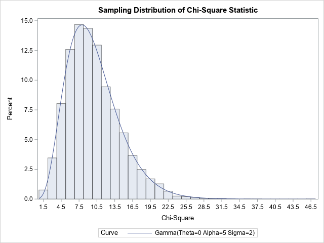
The histogram shows that a chi-square(10) distribution is a perfect fit for the sampling distribution of the chi-square statistic. As I explained in a previous article, this implies that the associated p-values are uniformly distributed. You can visualize this situation by plotting a histogram of the P_PCHI variable, as follows:

title "Distribution of P-Values for Hypothesis Test";
proc sgplot data=ChiSqStat;
   histogram P_PCHI / binwidth=0.05 binstart=0.025 scale=percent transparency=0.5;      /* center first bin at h/2 */
   refline 5 / axis=y;
run;

The p-values are uniformly distributed. This should give you confidence that the dice rolls are correctly simulated from the theoretical discrete probability distribution.

Summary

This article combines the ideas in two previous articles. In the first article, I showed how to simulate dice rolls in the SAS DATA step. In the second article, I showed that if data are simulated from a model for a hypothesis test, the p-values for the test are uniformly distributed. For simplicity, I showed that the p-values are uniformly distributed for a familiar hypothesis test of the mean of a continuous distribution. However, this article shows that the same ideas apply to some hypothesis tests for discrete distributions, provided that the test statistic is continuous.