A SAS statistical programmer recently asked a theoretical question about statistics. "I've read that 'p-values are uniformly distributed under the null hypothesis,'" he began, "but what does that mean in practice? Is it important?"

I think data simulation is a great way to discuss the conditions for which p-values are (or are not) uniformly distributed. This article does the following:

• Illustrate the conditions under which the p-values are uniformly distributed. Briefly, you must have a statistical model (M), a random sample (X) drawn from M, and a hypothesis test for which the test statistic has a known distribution.
• Illustrate a situation for which the p-values are no longer uniformly distributed. One common situation is when the model (M) and the data (X) have different distributions.

What are p-values anyway?

This section discusses some of the theory, use, and misuse of p-values. If you are familiar with p-value or just want to jump straight to an example, you can skip this section.

P-values can be a source of confusion, misinterpretation, and misuse. Even professional statisticians get confused. Students and scientists often don't understand them. It is for these reasons that the American Statistical Association (ASA) released a statement in 2016 clarifying the appropriate uses of p-values (Wasserman and Lazar, 2016, "The ASA Statement on p-Values: Context, Process, and Purpose", TAS). This statement was a response to several criticisms about how p-values are used in science. It was also a response to decisions by several reputable scientific journals to "ban" p-values in the articles that they publish.

I encourage the interested reader to read the six points in Wasserman and Lazar (2016) that describe interpretations, misinterpretations, applications, and misapplications of p-values.

The ASA statement on p-values is written for practitioners. Wasserman and Lazar (2016) define a p-value as follows: "Informally, a p-value is the probability under a specified statistical model that a statistical summary of the data (e.g., the sample mean difference between two compared groups) would be equal to or more extreme than its observed value." Under this definition, the p-value is one number that is computed by using one set of data. Unfortunately, this definition does not enable you to discuss the distribution of the p-value.

To discuss a distribution, you must adopt a broader perspective: You must think of a p-value as a random variable. This is discussed in the excellent article by Greenland (2019) and in the equally excellent article by Murdoch, Tsai, & Adcock (2008).

The idea is that the data (X) are a random sample from the assumed model distribution. When you generate a random sample, the data determines the test statistic for the null hypothesis. Therefore, the test statistic is a random variable. To each test statistic, there is a p-value. Therefore, the p-value, too, is a random variable. If the distribution of the test statistic is known, then the p-value is uniformly distributed, by definition, because it is the probability integral transform of the test statistic.

A simulation-based approach to p-values

This section shows a familiar example of a hypothesis test and a p-value: the one-sample t test for the mean. Recall that the one-sample t test assumes that a random sample contains independent draws from a normal distribution. (You can also use the t test for large samples from a non-normal continuous distribution, but, for simplicity, let's use normal data.) Assume that the data are drawn from N(72, σ). The null hypothesis is that H0: μ ≥ 72 versus the alternative hypothesis that μ < 72. Let's generate N=20 independent normal variates and use PROC TTEST in SAS to run the one-sided t test on the simulated data:

/* define the parameters */
%let N = 20;       /* sample size */
%let MU0 = 72;     /* true value of parameter */
data Sim1;         /* random sample from normal distrib with mu=&MU0 */
call streaminit(1234);
do i = 1 to &N;
   x = rand("Normal", &MU0, 10);
   output;
end;
run;
 
/* H0: generating distribution has mu<=&MU0. Since N is small, also assume data is normal. */
proc ttest data=Sim1 alpha=0.05 H0=&MU0 sides=L plots=none;
   var X;
run;

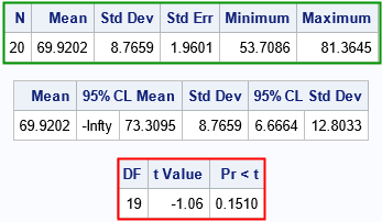
The output includes a table of descriptive statistics (the top table) for the sample. The middle table shows inferences about the parameters, such as that the true mean is probably less than 73.31. The last table is the one I want to focus on. It summarizes the test statistic for the hypothesis test. The test statistic has the value -1.06. Under the assumption that statistic is distributed according to the t distribution with 19 degrees of freedom, the probability that we would observe a value less than -1.06 is Pr(T < -1.06) = 0.1510.

Here's an important point: Since we simulated the data from the N(72, σ), we KNOW that the null hypothesis is true, and we know that the test statistics REALLY DOES have a T(DF=19) distribution! Therefore, we are not surprised when the t test has a large p-value and we fail to reject the null hypothesis.

Recall, however, that we might get unlucky when we simulate the sample. For 5% of normal samples, the t test will produce a small p-value and we will reject the null hypothesis. For that reason, when I check the correctness of a simulation, I like to generate many random samples, not just one.

A simulation study for the t test

If you want to understand the distribution of the p-values, you can perform a Monte Carlo simulation study in which you generate many random samples of size N from the same distribution. You run a t test on each sample, which generates many test statistics and many p-values. The following SAS program carries out this simulation study, as suggested by Murdoch, Tsai, & Adcock (2008):

/* simulation of many random samples */
%let NumSim = 10000;    /* number of random samples */
data SimH0;
call streaminit(1234);
do SampleID = 1 to &NumSim;
   do i = 1 to &N;
      x = rand("Normal", &MU0, 10);
      output;
   end;
end;
run;
 
ods exclude all;
proc ttest data=SimH0 alpha=0.05 H0=&MU0 sides=L plots=none;
   by SampleID;
   var X;
   ods output TTests=TTests;
run;
ods exclude none;
 
title "Test Statistics for One-Sample T-Test";
title2 "H0: mu0 <= &MU0";
proc sgplot data=TTests;
   histogram tValue / scale=percent transparency=0.5;
run;

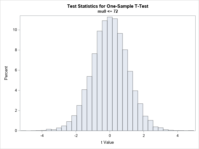
The data satisfy the assumptions of the t test and are sampled from a normal distribution for which the true parameter value satisfies the null hypothesis. Consequently, the histogram shows that the distribution of the test statistic looks very much like a t distribution with 19 degrees of freedom.

What does this have to do with p-values? Well, a p-value is just a transformation of a test statistic. The p-value is a way to standardize the test statistic so that it can be interpreted more easily. For any t, the corresponding left-tailed p-value is p = CDF("T", t, 29), or 1-CDF for a right-tailed p-value. As explained in an earlier article, if t is distributed as T(DF=29), then p is U(0,1). You can demonstrate that fact by plotting the p-values:

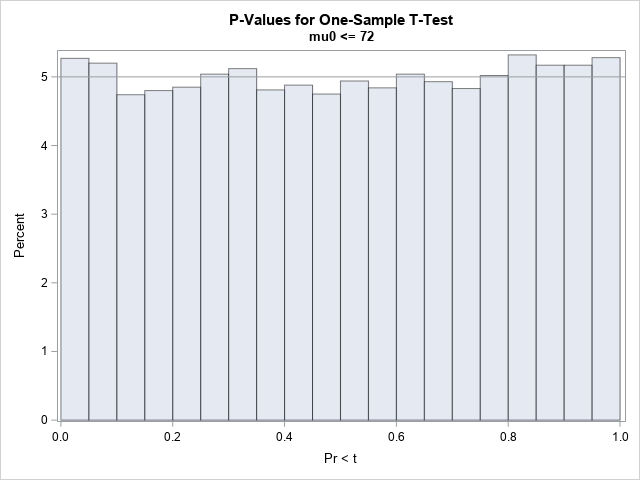
As promised, the p-values are uniformly distributed in (0,1). If you reject the null hypothesis when the p-value is less than 0.05, you will make a Type 1 error 5% of the time.

Notice that many things must happen simultaneously for the p-values to be uniformly distributed. The data must conform to the assumptions of the test and contain independent random variates from the model that is used to construct the test statistic. If so, then the test statistic follows a known t distribution. (Sometimes we only know an asymptotic distribution of the test statistic.) If all these stars align, then the p-values will be uniformly distributed.

When are the p-values NOT uniform?

If any of the previous assumptions are not true, then the p-values do not need to be uniformly distributed. The easiest situation to visualize is if the data are not sampled from a distribution whose mean equals the mean of the null hypothesis. For example, we generated the data from N(72, σ), but what happens if we run a t test for the hypothesis H0: μ ≥ 73? In this scenario, we expect more samples to reject the new null hypothesis. How many more? As suggested by Murdoch, Tsai, & Adcock (2008), we don't need to guess or compute, we can simply run the new hypothesis test for all 10,000 samples (which are from N(72, 10)) and plot the p-values:

/* what happens if the samples are NOT from the null hypothesis? */
%let MU1 = %sysevalf(1+&MU0);
ods exclude all;
proc ttest data=SimH0 alpha=0.05 H0=73 sides=L plots=none;
   by SampleID;
   var x;
   ods output TTests=TTestsNotH0;
run;
ods exclude none;
 
 
title "P-Values for One-Sample T-Test";
title2 "H0: mu = &MU0, but actually mu = &MU1";
proc sgplot data=TTestsNotH0;
   histogram probT / datalabel binwidth=0.05 binstart=0.025 /* center first bin at h/2 */
                     scale=percent transparency=0.5; 
   refline 5 / axis=y;
run;

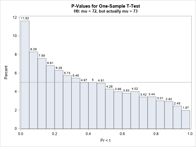
For the new hypothesis test, about 11.62% of the samples have a p-value that is less than 0.05. That means that if you use 0.05 as a cutoff value, you will reject the null hypothesis 11.62% of the time. This is good, because the samples are actually generated from a distribution whose mean is LESS than the hypothetical value of 73. In this case, the null hypothesis is false, so you hope to reject it. If you further increase the value used in the null hypothesis (try using 75 or 80!) the test will reject even more samples.

Summary

This article uses simulation to illustrate the oft-repeated assertion that "p-values are uniformly distributed under the null hypothesis." The article shows an example of a hypothesis test for a one-sample t test. When the data satisfy the assumptions of the t test and are generated so that the null hypothesis is correct, then the test statistic has a known sampling distribution. The p-value is a transformation of the test statistic. When the test statistic follows its assumed distribution, then the p-values are uniform. Otherwise, the p-values are not uniform, which means that using a p-value cutoff such as 0.05 will reject the null hypothesis with a probability that is different than the cutoff value.

For a second example, see "On the correctness of a discrete simulation."

Further reading

• Greenland, S. (2019), "Valid P-Values Behave Exactly as They Should: Some Misleading Criticisms of P-Values and Their Resolution With S-Values," TAS, 73, 106–114.
• Murdoch, D. J., Tsai, Y.-L., & Adcock, J. (2008), "P-Values are Random Variables," TAS, 62(3), 242–245.
• Wasserstein, R. L., & Lazar, N. A. (2016), "The ASA Statement on p-Values: Context, Process, and Purpose," TAS, 70(2), 129–133.