A previous article about standardizing data in groups shows how to simulate data from two groups. One sample (with n1=20 observations) is simulated from an N(15, 5) distribution whereas a second (with n2=30 observations) is simulated from an N(16, 5) distribution. The sample means of the two groups are close to each other: 14.9 and 15.15. In fact, if you run a t test on these data, the t test concludes that the samples probably came from populations that have the same mean parameter. More formally, the t test accepts (fails to reject) the null hypothesis that the two means are the same.

Making an incorrect inference like this is called a Type 2 error. Recall that the power of a statistical hypothesis test is the probability of rejecting the null hypothesis when the alternative hypothesis is true, which is 1 minus the probability of making a Type 2 error. This article uses PROC POWER to compute the exact power of a t test and then uses simulation to estimate the power. Along the way, I show a surprising and useful feature of SAS/IML programming.

Power and Type 2 errors

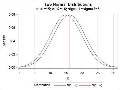
Let's run a t test on simulated data from normal distributions and let's only use SMALL sample sizes. The two normal distributions are shown to the right. The first sample is simulated from N(15,5) and the second sample is simulated from N(16,5). The distributions are close to each other, so a t test will not often infer that the samples are from different distributions. For this situation, the t test does not have much power.

The following SAS DATA step is the same as in the previous article. It simulates the data and calls PROC TTEST to analyze the data. (In this article, all tests are performed at the α=0.05 significance level.) The null hypothesis is that the group means are equal; the alternative hypothesis is that they are not equal. The data are simulated from distributions that have the same variance, so you can use the pooled t test to analyze the data.

/* Samples from N(15,5) and N(16, 5). */
%let mu1 = 15;
%let mu2 = 16;
%let sigma = 5;
data TwoSample;
call streaminit(54321);
n1 = 20; n2 = 30;
Group = 1;
do i = 1 to n1;
   x = round(rand('Normal', &mu1, &sigma), 0.01);  output;
end;
Group = 2;
do i = 1 to n2;
   x = round(rand('Normal', &mu2, &sigma), 0.01);  output;
end;
keep Group x;
run;
 
proc ttest data=TwoSample plots=none;
   class Group;
   var x;
run;

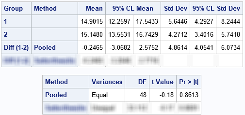
I blurred the rows of the tables that correspond to the Satterthwaite test so that you can focus on the pooled t test. The pooled test uses the difference between the sample means (-0.25) and the pooled standard deviation (4.86) to construct a t test for the difference of means. The p-value for the two-sided test is 0.8613, which means that the data do not provide enough evidence to reject the null hypothesis.

Because we simulated the data, we know that, in fact, the difference between the population means is not zero. In other words, the t test made a "Type 2" error: it failed to reject the null hypothesis even though the alternative hypothesis (unequal means) is true. The probability of a Type 2 error depends on the sample sizes and the magnitude of the effect you are trying to detect.

An exact computation of power

The power is 1 minus the probability of making a Type 2 error. A two-sample t test is one of the tests that is supported by PROC POWER in SAS. You can use PROC POWER to find the power of a t test for random samples of size n1=20 and n2=30 when the true difference between the means is 1.

/* compute exact power */
proc power;
  twosamplemeans  power = .           /* missing ==> "compute this" */
    meandiff= 1                       /* difference of means        */
    stddev=5                          /* N(mu1-mu2, 5)              */
    groupns=(20 30);                  /* num obs in the samples     */
run;

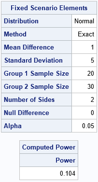
For these parameter values, the tables tell you that the two-sided t test will correctly reject the null hypothesis only 10% of the time (power=0.104) at the α=0.05 significance level. In 9 out of 10 random samples, the t test will (incorrectly) conclude that the sample comes from populations that have the same mean.

A simulation approach to estimate power in SAS/IML

I previously wrote about how to use simulation to estimate the power of a t test. That article shows how to use the DATA step to simulate many independent samples and then uses BY-group processing in PROC TTEST to analyze each sample. You use the ODS OUTPUT statement to capture the statistics for each analysis. The proportion of samples that reject the null hypothesis is an estimate of the power of the test.

If you can write a SAS/IML function that implements a t test, you can perform the same power computation in PROC IML. The following SAS/IML program (based on Chapter 5 of Wicklin (2013) Simulating Data with SAS) defines a function that computes the t statistic for a difference of means. The function returns a binary value that indicates whether the test rejects the null hypothesis. To test the function, I call it on the same simulated data:

proc iml;
/* SAS/IML function for a pooled t test.
   X : column vector with n1 elements from a population with mean mu_x. 
   Y : column vector with n2 elements from a population with mean mu_y.
   Compute the pooled t statistic for the difference of means and return whether 
   the statistic rejects the null hypothesis 
      H0: mu_x = mu_y
   at the alpha signif level. Formulas from the SAS documentation: https://bit.ly/30rr2GV
*/
start TTestH0(x, y, alpha=0.05);
   n1 = nrow(X);    n2 = nrow(Y);             /* sample sizes */
   meanX = mean(x); varX = var(x);            /* mean & var of each sample */
   meanY = mean(y); varY = var(y);
   DF = n1 + n2 - 2;
   /* pooled variance: https://blogs.sas.com/content/iml/2020/06/29/pooled-variance.html */
   poolVar = ((n1-1)*varX + (n2-1)*varY) / DF;
   /* Compute test statistic, critical value, and whether we reject H0 */
   t = (meanX - meanY) / sqrt(poolVar*(1/n1 + 1/n2));
   *print (meanX - meanY)[L="Diff (1-2)"] (sqrt(poolVar))[L="PoolSD"] t;
   t_crit = quantile('t', 1-alpha/2, DF); 
   RejectH0 = (abs(t) > t_crit);              /* binary 0|1 for 2-sided test */
   return RejectH0;                           
finish;
 
use TwoSample;
read all var 'x' into x where(group=1);
read all var 'x' into y where(group=2);
close;
 
reject = TTestH0(x, y);
print reject;

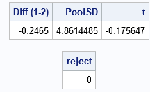
To confirm that the computations are the same as in PROC TTEST, I uncommented the PRINT statement in the module. The results are identical and the t test fails to reject the null hypothesis for these simulated data.

Notice that the SAS/IML function is both concise (less than 10 lines) and mimics the formulas that you see in textbooks or documentation. This "natural syntax" is one of the advantages of the SAS/IML language.

Simulation to estimate power in PROC IML

The SAS/IML function looks like a typical function for a univariate analysis, but it contains a surprise. Without making any modifications. you can call the function to run thousands of t tests. The module is written in a vectorized manner. If you send in matrices that have B columns, the module will run t tests for each column and return a binary row vector that contains B values.

Take a close look at the SAS/IML function. The MEAN and VAR functions operate on columns of a matrix and return row vectors. Consequently, the meanX, meanY, varX, and varY variables are row vectors. Therefore, the poolVar and t variables are also row vectors, and the RejectH0 variable is a binary row vector.

To demonstrate that the function can analyze many samples in a single call, the following statements simulate 100,000 random samples from the N(15,5) and N(16,5) distributions. Each column of the X and Y matrices is a sample. One call to the TTestH0 function computes 100,000 t tests. The "colon" subscript reduction operator computes the mean of the vector, which is the proportion of tests that reject the null hypothesis. As mentioned earlier, this is an estimate of the power of the test.

/* simulation of power */
B = 1e5;                  /* number of independent samples (number of cols) */
n1 = 20; n2 = 30;         /* sample sizes (number of rows) */
call randseed(321);
x = j(n1, B);             /* allocate array for samples from Group 1 */
y = j(n2, B);             /* allocate array for samples from Group 2 */
call randgen(x, 'Normal', &mu1, &sigma);   /* X ~ N(mu1,sigma) */
call randgen(y, 'Normal', &mu2, &sigma);   /* Y ~ N(mu2,sigma) */
reject = TTestH0(x, y);   /* result is row vector with B elements */
 
power = reject[:];
print power[L="Power (B=1E5)"];

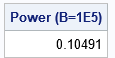
The result is very close to the exact power as computed by PROC POWER.

Notice also that the SAS/IML function, when properly written, can test thousands of samples as easily as it tests one sample. The program does not require an explicit loop over the samples.

Summary

This analysis starts with samples that are simulated from distributions that have different means. A t test fails to reject the null hypothesis (equal means) for 90% of the random samples. It draws the correct conclusion for about 10% of random samples, as shown by PROC POWER. You can estimate this value by simulating many samples and computing the proportion that rejects the null hypothesis. The simulation agrees with the exact power.

I previously wrote a simulation of power by using the DATA step and BY-group processing in PROC TTEST. But in this article, I implement a t test by writing a SAS/IML function. You might be surprised to discover that you can pass many samples to the function, which runs a test on each column of the input matrices.

It is worth mentioning that you can repeat this computation for many parameter values to obtain a power curve. For example, you can vary the difference between the means to determine how the power depends on the magnitude of the difference between the means.