Last week I showed how to use simulation to estimate the power of a statistical test. I used the two-sample t test to illustrate the technique. In my example, the difference between the means of two groups was 1.2, and the simulation estimated a probability of 0.72 that the t test would detect the difference.
Of course, the value 1.2 was completely arbitrary. You could just as well ask for the probability of detecting a difference of size 0.5, 1.0, or 2.0. You can repeat the simulation for any value of the difference and thereby construct a power curve. That's what I do in this article, which is based on material in Chapter 5 of Simulating Data with SAS.
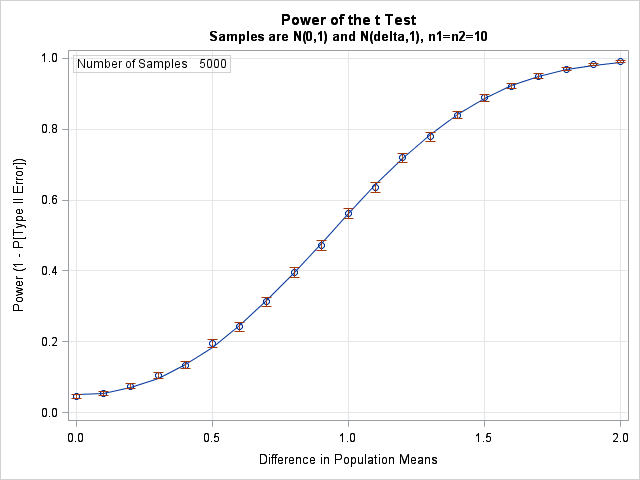
Here is the result of running the previous simulation for differences of size 0, 0.1, 0.2, ..., 2.0. The points along the curve are power estimates from the simulation, along with 95% confidence intervals. The size of the error bars reflects the number of simulations used for each point estimate, which is 5,000 for this simulation. The underlying curve is the result of running PROC POWER, which can solve this problem exactly. For more complicated statistical tests, an exact power curve is not available and simulation is the only way to estimate power.
The simulation takes about 30 seconds to run on a desktop PC from 2010. You can download the complete SAS program that runs the simulation. The program is virtually identical to the program I discussed last week, except that there is now a loop over the parameter that controls the mean difference (do Delta = 0 to 2 by 0.1), and I have included the Delta parameter in two BY statements.
A few comments about the power curve:
- In this simulation, the two populations have unit standard deviations. The graph shows that when the true difference between the means is 0.5, there is a 20% chance of detecting the difference with such a small sample size (n1=n2=10). The chance rises to 56% when the difference is 1. To have an 80% chance, the means must differ by about 1.35.
- When there is no difference between the population means, the graph shows that there is a 5% chance that the t test will reject the null hypothesis (which is that the means are equal). This is consistent with the fact that the test is performed at the α = 5% significance level.
- Notice that the confidence intervals for the power are smaller when the curve is flatter and larger when the curve is steeper. You can exploit this to make your simulations run faster by using fewer simulation trials in certain parameter ranges. See the Chapter 6, "Strategies for Efficient and Effective Simulation," of Simulating Data with SAS.
Download the program and experiment with changing the parameters. Change NumSamples to 1000 to make your experiments run faster. What does the curve look like when (n1=n2=20)?

4 Comments
Dears at SAS,
I was trying calculate sample size for a cluster randomized control trial which has two different intervention groups and one control group (totally three groups). Is there a different assumption in sample size calculation for multiple groups other than two population proportion or mean? Is Bonferroni correction the best assumption or simply shall I use the two population and distribute it for the three groups?
I was using a formula for cluster randomized controlled trail with unequal cluster size, however, I faced difficulties in getting ICC (rho) and Coefficient of variation (CV). I didn't get a paper citing ICC and coefficient of variation and even I couldn’t get figures which enable me to calculate these constants. I was trying to calculate the average cluster size using a fixed cluster number but when I did feasibility check, the assumption was not satisfied. Do you have some advice or recommendation?
Even different people say different; the published papers even didn’t have a uniform consensus. Some paper says as I should do a simulation to have a sample size with a good power other say different. I do have three outcome variables with count and binary outcome.
Could you support me how I do simulation to determine the required sample size for a cluster randomized controlled trial which has three groups? What steps should I follow on the SAS software to calculate or simulate sample size? Which program, under the installed application there are lots of options like SAS Enterprise Guide, SAS ILM Studio, etc, should I use?
I have two types of outcomes; binary and count. The sample size I want to determine should take into consideration the following issues;
1. cluster number
2. cluster size
3. coefficient of variation
4. intracluster correlation coefficient / rho and
5. effect size
in addition to individual randomized controlled trila.
How can I determine the sample size for three groups; is the Bonferroni correction appropraite for it or is it possible two use the two population formula and then allocate for the three groups or is there any correction assumption other than this that SAS will consider?
With kind regards
Teketo Kassaw
You can ask questions like this at the SAS Support Community for statistical procedures.
Dear colleagues, can you help me in calculation of sample size for four amr cluster randomized trial/
If you want to do this in SAS, you should post to the SAS Support Communities.